Model field particles with positional appearance learning for sports player tracking
Tam metin
Şekil
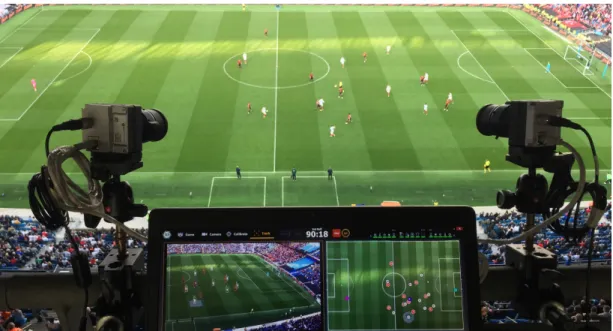
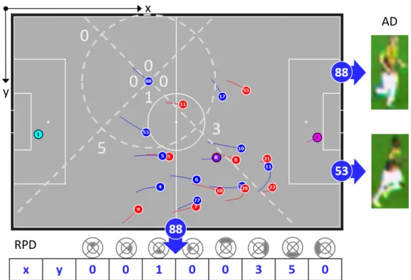
![Figure 1.1: Samples of analysis data provided in real-time by Sentio Sports An- An-alytics [3] to the soccer teams](https://thumb-eu.123doks.com/thumbv2/9libnet/5881713.121431/14.918.202.765.176.592/figure-samples-analysis-provided-sentio-sports-alytics-soccer.webp)
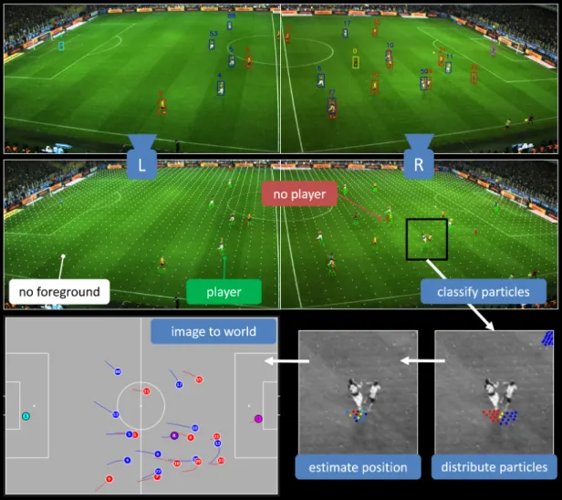
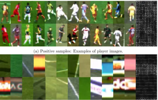
![Figure 3.5: Steps of player detection. Each particle having a ratio of foreground pixels above some threshold are considered as a candidate to contain a player, then f-HOG [55] features are extracted for these particles, and finally an SVM classifier is us](https://thumb-eu.123doks.com/thumbv2/9libnet/5881713.121431/32.918.188.776.170.541/detection-foreground-threshold-considered-candidate-extracted-particles-classifier.webp)
Benzer Belgeler
Fatehi &Masrori(2013) in a study with title” Analysis of the inhibiting factors and stimulating student participation in extracurricular sports programs” have
(36) demonstrated the presence of tonsillar biofilm producing bacteria in children with recurrent exacerbations of chronic tonsillar infections and suggested that tonsillar size is
Here, we study the nonequilibrium Hall response following a quench where the mass term of a single Dirac cone changes sign and apply these results to understanding quenches in
Considering both the calculations on the adsorption of a single Ir atom and measured STM images, we came up with a model of Ir-silicide nanowires (see Figure 4 ).. The local
Bu çalışmada, Balıkesir’de bulunan 3 kamu hastanesinin yoğun bakım ünitelerinde yatan hastalardan alınan rektal sürüntü örneklerinde VRE kolonizasyonu ile
HABER MERKEZİ REFAH Partili Kültür Ba kanı İsmail Kahraman, Taksim’e cami yapılmasına engel olarak görüp, görevden aldığı İstanbul 1 Numaralı Kültür ve
Şekil 2’ye göre, IFRS taksonomileri, işletmelerin finansal raporlarında yer alan bilgilerinin etiketlenmesinde kullanılmaktadır. Bu etiketleme işlevi ile birlikte
____dekorasyonda renk olarak Marakeş Mavisi'nin hakim olduğu lokantanın duvarlarında ahşap, hasır storlar kullanılmış. Safari dekoru ile Kuzey Afrika ağırlıklı bir
