Design of PD controlleers for unstable infinitive dimensional plants with time-delay

(1)

DESIGN OF PD CONTROLLERS FOR

UNSTABLE INFINITE DIMENSIONAL

PLANTS WITH TIME-DELAY

a thesis submitted to

the graduate school of engineering and science

of bilkent university

in partial fulfillment of the requirements for

the degree of

master of science

in

electrical and electronics engineering

By

Deniz Varol

(2)

DESIGN OF PD CONTROLLERS FOR UNSTABLE INFINITE DIMENSIONAL PLANTS WITH TIME-DELAY

By Deniz Varol June, 2015

We certify that we have read this thesis and that in our opinion it is fully adequate, in scope and in quality, as a thesis for the degree of Master of Science.

Prof. Dr. Hitay ¨Ozbay (Advisor)

Prof. Dr. ¨Omer Morg¨ul

Prof. Dr. Mehmet ¨Onder Efe

(3)

ABSTRACT

DESIGN OF PD CONTROLLERS FOR UNSTABLE

INFINITE DIMENSIONAL PLANTS WITH

TIME-DELAY

Deniz Varol

M.S. in Electrical and Electronics Engineering Advisor: Prof. Dr. Hitay ¨Ozbay

June, 2015

In real life, everything is in movement so there are always continuous trans-fers, transmissions and transports of people, materials, information and energy to other places. These transfers, transmissions and transports occur with a time delay. In control theory, time delays are encountered very commonly as in real life. By considering this fact, four unstable plants with time delays are considered from different application perspectives and five delay values are chosen. For stabi-lization of these infinite dimensional plants, PD controllers are designed by three different design methods: two of them give different least fragile PD controllers and the other design method gives a gain margin optimizing PD controller. De-signed PD controllers and equivalent plants are put in feedback loop and robust performance test results and step responses are obtained and compared.

(4)

¨

OZET

KARARSIZ SONSUZ BOYUTLU VE ZAMAN

GEC˙IKMEL˙I MODELLER ˙IC

¸ ˙IN PD KONTROLC ¨

U

TASARIMI

Deniz Varol

Elektrik ve Elektronik Mühendisli˘gi, Yüksek Lisans Tez Danı¸smanı: Prof. Dr. Hitay Özbay

Haziran, 2015

Ger¸cek hayatta her¸sey hareket halindedir, bu sebeple insanlar, e¸syalar, bilgiler ve enerjiler daimi olarak ba¸ska yerlere ta¸sınır, nakledilir ve iletilir. Bu ta¸sınımlar, iletimler ve nakiller sırasında bir miktar zaman kaybedilir ve bu kaybedilen za-man zaza-man gecikmesi olarak tanımlanır. Ger¸cek hayatta oldu˘gu gibi kontrol teorisinde de zaman gecikmeleri sık¸ca görülmektedir. Bu sebepten dolayı, dört adet zaman gecikmeli kararsız model olu¸sturulmu¸s ve be¸s tane zaman gecikme de˘geri se¸cilmi¸stir. Bu sonsuz boyutlu modellerin kararlı hale getirilebilmesi i¸cin ü¸c farklı tasarım yöntemi se¸cilmi¸stir: bu yöntemlerden ikisi en az kırılgan olan kontrolcüyü, di˘geri ise kazan¸c payı optimize eden kontrolcüyü vermekte-dir. Tasarlanan kontrolcüler ve kar¸sılık gelen modeller geri besleme döngüsüne yerle¸stirilmi¸s ve gürbüz performans testi ve step girdisine olan tepkileri elde edilmi¸s ve kar¸sıla¸stırılmı¸stır.

(5)

Acknowledgement

Firstly, I would like to express my deep gratitude to my supervisor, Prof. Dr. Hitay ¨Ozbay, for his patient guidance, effective suggestions and endless support throughout the master education and I would like to thank him for giving the opportunity of having this valuable education under his supervision.

I would like to thank Prof. Dr. ¨Omer Morg¨ul and Prof. Dr. Mehmet Mete ¨

Onder for being on my thesis committee.

I would also like to thank Bilkent University EE Department for their financial support.

In addition, I would like to express my thanks to my office mate Buket Koyuncu for sharing all the valuable times with me during the graduate studies and Mustafa Akın for his technical support.

Last but not least, I am grateful to my family Ayhan, Fehmiye and Barı¸s and my beloved companion Mustafa Mert Birincio˘glu for their incredible love, support and faith in me. Without them, I won’t be able to achieve this much.

(6)

List of Figures

1.1 Controller graph with delayed feedback from the output. . . 3

2.1 Feedback system. . . 6

3.1 Stabilizing Kp and Kd pairs for P1(s) when h = 0.1 sec. . . 12

(10)

LIST OF FIGURES x

3.22 amax(Q) versus Q graph for P2(s) when h is between 0.1 sec and 0.5 sec. . . 36

3.25 Stabilizing Kd(h) versus h graph when h is between 0.1-0.5 sec with design method-I. . . 55

3.26 Stabilizing Kp(h) versus h graph when h is between 0.1-0.5 sec with design method-I. . . 56

(11)

LIST OF FIGURES xi

3.28 Stabilizing Kp(h) versus h graph when h is between 0.1-0.5 sec

with design method-I. . . 58 3.29 Stabilizing Kd(h) versus h graph when h is between 0.1-0.5 sec

with design method-II. . . 58 3.30 Stabilizing Kp(h) versus h graph when h is between 0.1-0.5 sec

with design method-II. . . 59 3.31 Stabilizing Kd(h) versus h graph when h is between 0.1-0.5 sec

with design method-III. . . 59 3.32 Stabilizing Kp(h) versus h graph when h is between 0.1-0.5 sec

with design method-III. . . 60 3.33 Stabilizing Kd(h) versus h graph when h is between 0.1-0.5 sec

with design method-I. . . 61 3.34 Stabilizing Kp(h) versus h graph when h is between 0.1-0.5 sec

with design method-III. . . 63 3.37 Stabilizing Kd(h) versus h graph when h is between 0.1-0.5 sec

with design method-I. . . 65 3.38 Stabilizing Kp(h) versus h graph when h is between 0.1-0.5 sec

(12)

LIST OF FIGURES xii

3.40 Stabilizing Kp(h) versus h graph when h is between 0.1-0.5 sec

with design method-II. . . 66 3.41 Stabilizing Kd(h) versus h graph when h is between 0.1-0.5 sec

with design method-III. . . 67

4.1 Step response of the feedback system with plant P1(s) and the

controller C(s) in (3.2) when h = 0.1 sec. . . 74 4.2 Step response of the feedback system with plant P1(s) and the

(13)

LIST OF FIGURES xiii

(14)

LIST OF FIGURES xiv

controller C(s) in (3.74) when h = 0.4 sec. . . 92 4.33 Step response of the feedback system with plant P (s) and the

(15)

LIST OF FIGURES xv

(16)

List of Tables

3.1 Obtained PD Controllers for P1(s) with Design Method-I . . . 55

3.2 Allowable Ranges for Kp by Design Method I and II for P2(s) . . 57

3.3 Obtained PD Controllers for P2(s) . . . 57

4.1 Robust Performance Test Results for P1(s) with PD Controllers

Obtained from Design Method-I . . . 71 4.2 Robust Performance Test Results for P3(s) and P4(s) . . . 72

(17)

Chapter 1 INTRODUCTION

In real life, everything is in movement so there are always continuous transfers, transmissions and transports of people, materials, information and energy to other places. These transfers, transmissions and transports occur with a time delay. In control theory, time delays are encountered very commonly. In this thesis, several unstable plants with time delays are investigated and stabilized by various PD controllers.

1.1 Scope of the Thesis

In this thesis, there are three stages of studies:

(i ) selecting four different plants whose structures are frequently encountered in control area,

(ii ) designing PD controllers with three design methods,

(iii ) robustness and performance comparison of the feedback system under these controllers.

For the first step, commonly used and modelled plant structures in practical life are searched. After that, four plant structures are generated among encountered

(18)

These plants are unstable plants with five different chosen time delay values, so in total, twenty different version of plants are obtained.

For the second step, design of least fragile PD controllers with two different methods and design of gain margin optimizing PD contollers are investigated. These methods are chosen because of their functionality as fragility and gain margin are vital properties for control systems. Moreover, PD controllers are used in many practical applications for ease of their implementation.

Finally, for the last step robustness is checked by using robust performance condition as plants and controllers are fixed after the PD controllers are designed. Also, for comparing the time tracking performances of the designed feedback systems, step responses are obtained and compared.

1.2 Related Work

Significant amount of control systems include unstable plants and stabilization of these systems with controllers have a vital role in all areas, especially in engineer-ing systems. Because of this fact, many researchers developed various controller design methods.

Some of the most frequently used controller design methods are P, PD, PI and PID controllers [2, 3, 4], LQR (Linear Quadratic Regulator) control design [5], Smith predictor design [6, 7], IMC (Internal Model Control) [8, 9], Taylor or Pad´e Approximation [10], H∞optimal control design [11] and so forth. However,

many of these methods have some restrictions and cannot be applied to all types of plants. For example, LQR control design method can be only applied to the systems without time delays as in [5]. Its extension to infinite dimensional systems is possible but not very practical [12]. Other examples are the Smith predictor design and IMC, which are used with only stable open loop plants with time

(19)

Design of P, PD, PI and PID controllers, Taylor approximation, Pad´e approx-imation and H2/H∞ optimal control design can be used with unstable plants

with time delays without restrictions. Many of the approximation based con-trollers require relatively small time delays. Typically state space based methods require complex computations that may lead to fragile controllers. PI and PID controllers are used frequently with unstable systems with small or large time de-lays. But PD controllers are used less frequently (mainly when the plant contains an integral action).

After considering all of the related works, in this thesis, design of PD controllers for the unstable plants with time delay is selected between them for stabilization because of the simplicity of the control structure. In addition, in the literature there is relatively less research on PD controllers (compared to P, PI and PID controllers) on plants with large time delays.

1.3 On PD Controllers

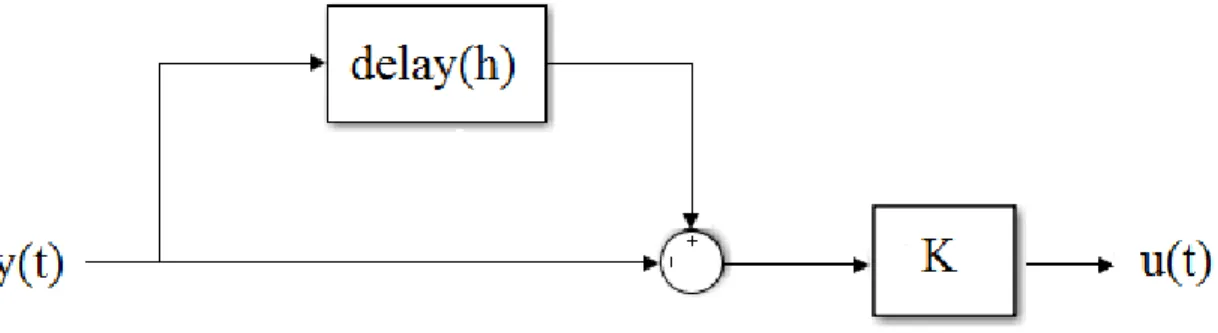
Let us consider a controller with delayed feedback from the output as shown in the Figure 1.1

(20)

and chaos control schemes and such a control scheme is studied in [13], [14] and [15]:

u(t) = −Ky(t) + Ky(t − h). (1.1)

According to fundamental theorem of calculus

˙

f (a) = lim

h→0

f (a + h) − f (a)

h , (1.2)

so for small h values

˙

f (a) = f (a + h) − f (a)

h . (1.3)

After considering (1.3), (1.1) can be written as:

u(t) = −K(y(t) − y(t − h)) = −Kh(y(t)−y(t−h)_h ) = −Kh ˙y(t).

It can be easily seen u(t) is a derivative controller. As derivative controllers have rare usage, are not practical controllers and are not able to stabilize most of the plants, a new approach is investigated and a modification to u(t) is decided.

For having a new approach, u(t) is modified as:

u(t) = −K1y(t) + K2y(t − h)

= −K1y(t) + K2y(t − h) + K2y(t) − K2y(t)

= −K2[y(t) − y(t − h)] + (K2− K1)y(t)

= −K2h ˙y(t) + (K2− K1)y(t).

(21)

It can be concluded that when K1 and K2 are used instead of one K in (1.1),

PD controller can be obtained for small h values. As small h values must be used, h is selected between 0.1 sec and 0.5 sec.

By using different K1 and K2 values desired Kd and Kp pairs can be obtained

so modified u(t) can be directly accepted as PD controller. Because of this fact, K1 and K2 are not going to be mentioned after this section, i.e., instead Kd and

Kp values are going to be calculated directly.

1.4 Organization of the Thesis

The thesis starts with Chapter 2 where problem definition is included. Problem definition is divided into two as feedback system stability and controller structure and plant types. The structure of PD controllers and feedback loop are explained and the chosen plants are stated. In Chapter 3, three PD controller design meth-ods are defined, applied to the plants and PD controllers are obtained and listed. Chapter 4 includes all simulations and results where robust performance results and step responses are given. In Chapter 5, conclusion and future works are stated. Last but not least, Appendix 1 includes all Matlab codes which are used in the process of preparing the thesis.

(22)

Chapter 2 PROBLEM DEFINITION

2.1 Feedback System Stability and Controller

Structure

The feedback system formed by the controller C and the plant P as in Figure 2.1 is stable if

(i) S := (1 + P C)−1 (ii) CS

(23)

If these conditions hold, then the controller C is said to stabilize the plant P . In order to achieve stabilization of the plants, PD controllers are used in this thesis; they are first order controllers in the form:

Cpd(s) = Kds + Kp where Kd is derivative gain and Kp is proportional gain.

This thesis aims to obtain the stabilizing Kd and Kp pairs, gain margin

op-timizing and least fragile PD controllers for four various plants by three design methods. The chosen plants are explained in the next section in detailed way.

2.2 Plant Types

Unstable processes with time delays have many different structures with differ-ent amount of orders. Most of the chemical systems, biological and engineering systems such as continuously stirred tank reactors, polymerization reactors, biore-actors and computer communication networks inherently have unstable behaviour and contain time delay because of measurement delay or the approximation of higher order dynamics of the process. Most of these systems are modeled as un-stable first order processes with time delays (UFOPTD), unun-stable second order processes with time delays (USOPTD) and unstable third order processes with time delays (UTOPTD) [17, 18]. Some plant structures which have UFOPTD, USOPTD and UTOPTD are as follows.

Unstable first order processes with time delays mostly have the plant structure:

P (s) = Ke

−hs

s − a (2.1)

where h > 0, K > 0 and a ≥ 0.

Some processes which have this structure are control of the high frequency longitudinal dynamics (short period) of an aircraft [19] and batch chemical reactor

(24)

[20].

Unstable second order processes with time delays mostly have the plant struc-ture:

P (s) = Ke

−hs

(s − a)(s + b) (2.2)

where h > 0, K > 0, a ≥ 0 and b can be both negative, positive or 0.

The temperature control in the heated tank of a pilot plant can be given as example where USOPTD are used [21].

Unstable third order processes with time delays mostly have the plant struc-ture:

Ke−hs

(s − a)(s + b)(s + c) (2.3)

where h > 0, K > 0 and a ≥ 0 and b, c can be both negative, positive or 0. Third order unstable processes can be encountered in control of tank reactors. In stabilization of the continuously stirred tank reactor (CSTR), the transfer function between concentration of the product and cooling liquid temperature at the input is an example for UTOPTD [22].

After investigating most encountered unstable plant types with time delays four plants are chosen to be used in this thesis. One second order and three third order unstable plants with time delays are selected as there are many researches on first order plants [23, 24, 25, 26, 27]. In addition, when a process is higher order (more than third order), in many practical applications it can be reduced to first order, second order and third order process models by using the model reduction methods [28]. The chosen plants are:

(25)

2. P2(s) = e−hs (s − 0.5)(s2_{+ s + 1)} = e−hs s3_{+ 0.5s}2_{+ 0.5s − 0.5} 3. P3(s) = e−hs s(s2_{+ s + 1)} = e−hs s3_{+ s}2_{+ s} 4. P4(s) = e−hs (s − 10−3_)(s2_{+ s + 1)} = e−hs s3 _{+ 0.999s + 0.999 − 0.001}

where h is the time delay amount and h > 0. Different h values are used in order to see the effect of various time delays: h = 0.1; 0.2; 0.3; 0.4; 0.5 sec.

The first plant P1(s) is USOPTD and have two unstable poles. The plant

is designed as an integrating process with one pole at origin and one pole at right half plane because integrating processes are very frequently encountered in process industries and considerable numbers of chemical processes can be modeled as integrating processes with time delay [25].

The other plant models, P2(s), P3(s) and P4(s) only differ in the unstable

pole. The plants are chosen in this way because the effect of the location of the unstable pole to PD controllers is desired to be investigated. The unstable pole of P3(s) and P4(s) are intentionally selected very close. The reason for this is

(26)

Chapter 3 DESIGN OF PD

CONTROLLERS

Three design methods are used to find the PD controllers (Kd and Kp values)

which stabilize the plants. For each plant P1(s), P2(s), P3(s) and P4(s),

sepa-rate PD controller sets are found, i.e., design methods are applied to each plant individually. First design method provides the least fragile PD controller via allmargin command of MATLAB, second design method provides gain margin optimizing PD controller and third design method provides another least frag-ile PD controller. Second and third design methods are taken from the ”PD Controller Design” section of [1].

3.1 Design Method-I: Design of Least Fragile

PD Controllers

Fragility of a controller refers to violation of the feedback system stability by per-turbations in the controller parameters (see [29],[30]). In order to find the least

(27)

command of MATLAB to find the stabilizing PD controller sets. The allmargin command computes gain margin, phase margin, delay margin and stability of a SISO open-loop model. This SISO open-loop model must be in the transfer function form and must not have time delay in the denominator so all four plants P1(s), P2(s), P3(s) and P4(s) are suitable for this design method. As allmargin

command uses open-loop model, P (s)C(s) is used as the SISO open-loop model. For different PD controllers (for different Kdand Kp pairs), allmargin command

is used and the stability of the feedback system is examined. If the command results with ”Stable:1”, then it means feedback system is stable and that PD controller C stabilizes the plant P . Whereas, if the command results with ”Sta-ble:0”, then it means that feedback system is not stable and that PD controller C does not stabilize the plant P .

In this design method, all PD controllers which stabilize each plant are recorded and indicated on the Kp-Kd plane. After that, the center point of each feasible

region is found by drawing the largest circle which fits inside the stability region. The center point gives the least fragile PD controller parameters, because it is the farthest point to the stability-instability boundary. Also, the allowable ranges for Kp are observed for P2(s), P3(s), P4(s) and will be compared with the ranges

which are obtained by design method-II. For finding the allowable ranges of Kp,

the minimum and the maximum values of Kp are obtained from the graphs and

(28)

3.1.1 Least Fragile PD Controllers for P

1

(s)

1. For h = 0.1 sec.

P1(s) =

e−0.1s

s(s − 0.5). (3.1)

The Kp and Kd pairs which stabilize P1(s) given in (3.1) are shown in

Fig-ure 3.1. 0 2 4 6 8 10 12 14 16 0 10 20 30 40 50 60 X: 9.5 Y: 25.1 K d K p K

p versus Kd graph for h=0.1

Figure 3.1: Stabilizing Kp and Kd pairs for P1(s) when h = 0.1 sec.

As can be seen from the figure, least fragile PD controller is:

C(s) = 9.5s + 25.1. (3.2)

After finding the stabilizing Kd and Kp pairs, another stability condition is

(29)

According to the stability condition, the phase margin should be positive, so the phase of P (jw)C(jw) should satisfy:

tan−1( ˜Kdwc) − π 2 − π + tan −1 (wc p ) − hwc> −π (3.3) where p = 0.5, ˜Kd = Kd Kp

and wc is the gain crossover frequency.

Note that (3.3) can be written as: tan−1( ˜Kdwc) + tan−1(

wc

p ) − hwc> π

2. (3.4)

The gain crossover frequency is computed from

| P (jw)C(jw) |= 1, (3.5) i.e., Kp q (1 + ˜K2 dwc2) wcpw2c+ p2 = 1. (3.6)

By taking square of both sides we obtain: K_p2(1 + ˜K_d2wc2) = w2c(w

2 c + p

2₎ _(3.7)

w_c4+ (p2− K_p2K˜_d2)w_c2− K_p2 = 0. (3.8)

As wc should be positive, the root which solves (3.8) is:

wc= s K2 d − p2 2 + r (K 2 d − p2 2 ) 2_{+ K}2 p. (3.9)

Since wc depends on Kd and Kp, it can be written as wc(Kd, Kp), then (3.4)

(30)

In conclusion, the positive phase margin condition is: tan−1( Kd r K2 d−p2 2 + q (K2d−p2 2 ) 2_{+ K}2 p Kp ) + tan−1( r K2 d−p2 2 + q (K2d−p2 2 ) 2_{+ K}2 p p ) − h s K2 d− p2 2 + r (K 2 d− p2 2 ) 2_{+ K}2 p> π 2. (3.11) The pairs (Kd, Kp) which satisfy this inequality are recorded and the obtained

region is shown in Figure 3.2:

0 2 4 6 8 10 12 14 16 0 10 20 30 40 50 60 K

p versus Kd graph for h=0.1

K

d

K p

As can be seen all Kd and Kp pairs match exactly the ones which are found

by allmargin command so it can be concluded that this design method is valid for finding stabilizing Kd and Kp pairs.

2. For h = 0.2 sec.

P1(s) =

e−0.2s

(31)

The Kp and Kd pairs which stabilize P1(s) given in (3.12) are shown in

Fig-ure 3.3.

C(s) = 4.7s + 5.78. (3.13)

3. For h = 0.3 sec.

P1(s) =

e−0.3s

(32)

The Kp and Kd pairs which stabilize P1(s) given in (3.14) are shown in Fig-ure 3.4. 0.5 1 1.5 2 2.5 3 3.5 4 4.5 5 0 0.5 1 1.5 2 2.5 3 3.5 4 4.5 5 X: 3.1 Y: 2.3 K d K p versus Kd for h=0.3 K p

C(s) = 3.1s + 2.3. (3.15)

4. For h = 0.4 sec.

P1(s) =

e−0.4s

(33)

The Kp and Kd pairs which stabilize P1(s) given in (3.16) are shown in Figure 3.5. 0.5 1 1.5 2 2.5 3 3.5 4 0 0.5 1 1.5 2 2.5 X: 2.305 Y: 1.15 K d K p K p versus Kd for h=0.4

C(s) = 2.305s + 1.15. (3.17)

5. For h = 0.5 sec.

P1(s) =

e−0.5s

(34)

The Kp and Kd pairs which stabilize P1(s) given in (3.18) are shown in Figure 3.6. 0.5 1 1.5 2 2.5 3 0 0.2 0.4 0.6 0.8 1 1.2 1.4 X: 1.85 Y: 0.68 K d K p K p versus Kd for h=0.5

C(s) = 1.85s + 0.68. (3.19)

3.1.2 Least Fragile PD Controllers for P

2

(s)

1. For h = 0.1 sec.

P2(s) =

e−0.1s

(35)

The Kp and Kd pairs which stabilize P2(s) given in (3.20) are shown in Figure 3.7. 0 0.5 1 1.5 2 2.5 3 3.5 4 4.5 5 0 0.2 0.4 0.6 0.8 1 1.2 1.4 X: 2.35 Y: 0.87 K d K p K p versus Kd for h=0.1

C(s) = 2.35s + 0.87. (3.21)

The allowable range for Kp:

0.5 < Kp < 1.23.

2. For h = 0.2 sec.

P2(s) =

e−0.2s

(36)

The Kp and Kd pairs which stabilize P2(s) given in (3.22) are shown in Figure 3.8. 0 0.5 1 1.5 2 2.5 3 0 0.1 0.2 0.3 0.4 0.5 0.6 0.7 0.8 0.9 1 X: 1.14 Y: 0.71 K d K p K p versus Kd for h=0.2

C(s) = 1.14s + 0.71. (3.23)

0.5 < Kp < 0.91.

3. For h = 0.3 sec.

P2(s) =

e−0.3s

(37)

The Kp and Kd pairs which stabilize P2(s) given in (3.24) are shown in Figure 3.9. 0 0.2 0.4 0.6 0.8 1 1.2 1.4 1.6 1.8 0 0.1 0.2 0.3 0.4 0.5 0.6 0.7 0.8 0.9 X: 0.76 Y: 0.65 K p versus Kd for h=0.3 K d K p

C(s) = 0.76s + 0.65. (3.25)

0.5 < Kp < 0.8.

4. For h = 0.4 sec.

P2(s) =

e−0.4s

(38)

The Kp and Kd pairs which stabilize P2(s) given in (3.26) are shown in Figure 3.10. 0 0.2 0.4 0.6 0.8 1 1.2 1.4 0 0.1 0.2 0.3 0.4 0.5 0.6 0.7 0.8 X: 0.6 Y: 0.63 K d K p K p versus Kd for h=0.4

C(s) = 0.6s + 0.63. (3.27)

0.5 < Kp < 0.74.

5. For h = 0.5 sec.

P2(s) =

e−0.5s

(39)

The Kp and Kd pairs which stabilize P2(s) given in (3.28) are shown in Figure 3.11. 0 0.2 0.4 0.6 0.8 1 1.2 1.4 0 0.1 0.2 0.3 0.4 0.5 0.6 0.7 0.8 X: 0.51 Y: 0.61 K p versus Kd for h=0.5 K d K p

C(s) = 0.51s + 0.61. (3.29)

0.5 < Kp < 0.71.

3.1.3 Least Fragile PD Controllers for P

3

(s)

1. For h = 0.1 sec.

(40)

The Kp and Kd pairs which stabilize P3(s) given in (3.30) are shown in Figure

3.12.

C(s) = 4.76s + 1.48. (3.31)

0 < Kp < 2.9.

2. For h = 0.2 sec.

P3(s) =

e−0.2s

(41)

The Kp and Kd pairs which stabilize P3(s) given in (3.32) are shown in Figure 3.13. 0 1 2 3 4 5 6 0 0.2 0.4 0.6 0.8 1 1.2 1.4 1.6 1.8 X: 2.24 Y: 0.83 K p versus Kd for h=0.2 K d K p

C(s) = 2.24s + 0.83. (3.33)

0 < Kp < 1.65.

3. For h = 0.3 sec.

P3(s) =

e−0.3s

(42)

The Kp and Kd pairs which stabilize P3(s) given in (3.34) are shown in Figure 3.14. 0 0.5 1 1.5 2 2.5 3 3.5 4 0 0.2 0.4 0.6 0.8 1 1.2 1.4 X: 1.42 Y: 0.62 K p versus Kd for h=0.3 K d K p

C(s) = 1.42s + 0.62. (3.35)

0 < Kp < 1.24.

4. For h = 0.4 sec.

P3(s) =

e−0.4s

(43)

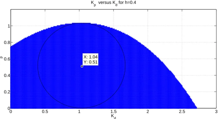
The Kp and Kd pairs which stabilize P3(s) given in (3.36) are shown in Figure 3.15. 0 0.5 1 1.5 2 2.5 3 0 0.2 0.4 0.6 0.8 1 X: 1.04 Y: 0.51 K p versus Kd for h=0.4 K d K p

C(s) = 1.04s + 0.51. (3.37)

0 < Kp < 1.03.

5. For h = 0.5 sec.

P3(s) =

e−0.5s

(44)

The Kp and Kd pairs which stabilize P3(s) given in (3.38) are shown in Figure 3.16. 0 0.5 1 1.5 2 2.5 0 0.1 0.2 0.3 0.4 0.5 0.6 0.7 0.8 0.9 1 X: 0.8 Y: 0.45 K p versus Kd for h=0.5 K d K p

C(s) = 0.8s + 0.45. (3.39)

0 < Kp < 0.91.

(45)

The Kp and Kd pairs which stabilize P4(s) given in (3.40) are shown in Figure

3.17.

C(s) = 4.7s + 1.44. (3.41)

0.001 < Kp < 2.89.

2. For h = 0.2 sec.

P4(s) =

e−0.2s

(46)

The Kp and Kd pairs which stabilize P4(s) given in (3.42) are shown in Figure 3.18. 0 1 2 3 4 5 6 0 0.2 0.4 0.6 0.8 1 1.2 1.4 1.6 1.8 X: 2.25 Y: 0.83 K p versus Kd for h=0.2 K d K p

C(s) = 2.25s + 0.83. (3.43)

0.001 < Kp < 1.65.

3. For h = 0.3 sec.

P4(s) =

e−0.3s

(47)

The Kp and Kd pairs which stabilize P4(s) given in (3.44) are shown in Figure 3.19. 0 0.5 1 1.5 2 2.5 3 3.5 4 0 0.2 0.4 0.6 0.8 1 1.2 1.4 X: 1.43 Y: 0.62 K d K p K p versus Kd for h=0.3

C(s) = 1.43s + 0.62. (3.45)

0.001 < Kp < 1.24.

4. For h = 0.4 sec.

P4(s) =

e−0.4s

(48)

The Kp and Kd pairs which stabilize P4(s) given in (3.46) are shown in Figure 3.20. 0 0.5 1 1.5 2 2.5 3 0 0.2 0.4 0.6 0.8 1 X: 1.04 Y: 0.51 K p versus Kd for h=0.4 K d K p

C(s) = 1.04s + 0.51. (3.47)

0.001 < Kp < 1.03.

5. For h = 0.5 sec.

P4(s) =

e−0.5s

(49)

The Kp and Kd pairs which stabilize P4(s) given in (3.48) are shown in Figure 3.21. 0 0.5 1 1.5 2 2.5 0 0.1 0.2 0.3 0.4 0.5 0.6 0.7 0.8 0.9 1 X: 0.79 Y: 0.45 K p versus Kd for h=0.5 K d K p

C(s) = 0.79s + 0.45. (3.49)

(50)

3.2 Design Method-II: Design of Gain Margin

Optimizing PD Controllers Given in [1]

This design method which is defined in [1] is only applicable to the plants which have the form:

P (s) = 1

s − pG(s) where p ≥ 0 is the unstable pole and G ∈ H∞ is the stable part of the plant.

G(s) can be irrational, i.e., P (s) can be infinite dimensional.

As P1(s) has two unstable poles, this design method is not applicable to P1(s).

The other plants P2(s), P3(s) and P4(s) satisfy this condition so gain margin

optimizing PD controllers are found for only three of the plants. According to [1], the structure of PD controller is defined as:

Cpd(s) = KpC0(s) where C0(s) = (1 + ˜Kds) so

Cpd(s) = ( ˜KdKp)s + Kp.

As Cpd(s) = Kds + Kp then Kd= ˜KdKp. In the analysis below ˜Kd is denoted

as a free parameter Q ∈ R.

The first step of the design method is determining an admissable Q interval for stability:

(51)

After defining the range for Q, for each Q in this interval, the largest a value (amax(Q)) should be found which satisfies the inequality:

(p + a) < 1 γ(Q, a) ∀ a < amax(Q) where γ(Q, a) :=k G0(s) − 1 s + a + Q s s + aG0(s) k∞ and G0(s) = G(s)G(0) −1 .

The next step is plotting amax(Q) versus Q and finding the maximum value of

amax(Q) and defining:

Qopt := arg max {amax(Q)}.

After finding the value of Qopt, the allowable range of the controller gain Kp can

be found by:

pG(0)−1 < Kp < (p + a0)G(0)−1 where

a0 := amax(Qopt). (3.50)

In conclusion, for p > 0, gain margin optimizing PD controller parameters are defined as: ˜ Kd,opt = Qopt Kp,GM opt = p p(p + a0)G(0)−1. So as Kd= ˜KdKp; Kd becomes

(52)

3.2.1 Gain Margin Optimizing PD Controllers for P

2

(s)

Obtained amax(Q) versus Q graph for P2(s) for h values between 0.1 sec and 0.5

sec and maximum amax(Q) points for each h are shown in Figure 3.22.

0 0.2 0.4 0.6 0.8 1 1.2 1.4 1.6 1.8 2 0 0.1 0.2 0.3 0.4 0.5 0.6 0.7 X: 0.9009 Y: 0.185 a

max(Q) versus Q for Different h Values

Q a m a x (Q) X: 0.904 Y: 0.239 X: 0.9653 Y: 0.306 X: 0.9991 Y: 0.396 X: 1.001 Y: 0.519 h=0.1 h=0.2 h=0.3 h=0.4 h=0.5

Figure 3.22: amax(Q) versus Q graph for P2(s) when h is between 0.1 sec and 0.5

sec. As it is stated P2(s) = e−hs (s − 0.5)(s2_{+ s + 1)} so p = 0.5 and G(s) = e −hs (s2_{+ s + 1)} G(0) = 1. 1. For h = 0.1 sec.

(53)

The allowable range of the controller gain Kp is:

0.5 < Kp < 1.019.

Gain margin optimizing PD controller parameters are:

Kp,GM opt =

p

0.5(0.5 + 0.519) = 0.714 Kd,GM opt= QoptKp,GM opt = 1.001 × 0.714 = 0.715.

So, the gain margin optimizing PD controller is:

C(s) = 0.715s + 0.714. (3.51)

2. For h = 0.2 sec.

Qopt = 0.9991 and a0 = 0.396.

0.5 < Kp < 0.896.

Kp,GM opt =

p

C(s) = 0.669s + 0.669. (3.52)

(54)

0.5 < Kp < 0.806.

Kp,GM opt =

p

C(s) = 0.613s + 0.635. (3.53)

4. For h = 0.4 sec.

Qopt = 0.904 and a0 = 0.239.

0.5 < Kp < 0.739.

Kp,GM opt =

p

(55)

5. For h = 0.5 sec.

Qopt = 0.9009 and a0 = 0.185.

0.5 < Kp < 0.685.

Kp,GM opt =

p

(56)

3.2.2 Gain Margin Optimizing PD Controllers for P

3

(s)

sec and maximum amax(Q) points for each h are shown in Figure 3.23.

0 0.2 0.4 0.6 0.8 1 1.2 1.4 1.6 1.8 2 0.8 1 1.2 1.4 1.6 1.8 2 X: 0.81 Y: 0.905 Q a m a x (Q) a

X: 0.85 Y: 1.005 X: 0.87 Y: 1.141 X: 0.91 Y: 1.335 X: 0.94 Y: 1.649 h=0.1 h=0.2 h=0.3 h=0.4 h=0.5

sec. As it is stated P3(s) = e−hs s(s2_{+ s + 1)} so p = 0 and G(s) = e −hs (s2_{+ s + 1)} G(0) = 1.

(57)

optimizing PD controllers. Same gain margin optimizing PD controllers will be used for P3(s) and P4(s) in Chapter 5.

1. For h = 0.1 sec.

Qopt = 0.94 and a0 = 1.649.

0 < Kp < 1.649.

2. For h = 0.2 sec.

Qopt = 0.91 and a0 = 1.335.

0 < Kp < 1.335.

3. For h = 0.3 sec.

Qopt = 0.87 and a0 = 1.141.

0 < Kp < 1.141.

(58)

0 < Kp < 1.005.

5. For h = 0.5 sec.

Qopt = 0.81 and a0 = 0.905.

0 < Kp < 0.905.

3.2.3 Gain Margin Optimizing PD Controllers for P

4

(s)

(59)

0 0.2 0.4 0.6 0.8 1 1.2 1.4 1.6 1.8 2 0.8 1 1.2 1.4 1.6 1.8 2 X: 0.8 Y: 0.904 a

Q a m a x (Q) X: 0.85 Y: 1.004 X: 0.88 Y: 1.138 X: 0.9 Y: 1.333 X: 0.94 Y: 1.646 h=0.1 h=0.2 h=0.3 h=0.4 h=0.5

sec. As it is stated P4(s) = e−hs (s − 10−3_)(s2_{+ s + 1)} so p = 10−3 = 0.001 and G(s) = e −hs (s2 _{+ s + 1)} G(0) = 1. 1. For h = 0.1 sec. Qopt = 0.94 and a0 = 1.646.

(60)

Kp,GM opt =

p

C(s) = 0.038s + 0.041. (3.56)

2. For h = 0.2 sec.

Qopt = 0.9 and a0 = 1.333.

0.001 < Kp < 1.334.

Kp,GM opt =

p

C(s) = 0.033s + 0.037. (3.57)

(61)

0.001 < Kp < 0.139.

Kp,GM opt =

p

C(s) = 0.03s + 0.034. (3.58)

4. For h = 0.4 sec.

Qopt = 0.85 and a0 = 1.004.

0.001 < Kp < 1.005.

Kp,GM opt =

p

(62)

5. For h = 0.5 sec.

Qopt = 0.8 and a0 = 0.904.

0.001 < Kp < 0.905.

Kp,GM opt =

p

0.001(0.001 + 0.905) = 0.03 Kd,GM opt = QoptKp,GM opt = 0.8 × 0.03 = 0.024.

C(s) = 0.024s + 0.03. (3.60)

3.3 Design Method-III: Design of a PD

Con-troller Minimizing Fragility in the

Propor-tional Gain Given in [1]

In [1] derivative action ˜Kd = Kd/Kp = Q is optimized so that allowable region

for the proportional gain is maximized, and the midpoint of this region is selected so that least fragile proportional gain is used in the controller. The following is a brief summary of the steps for calculating this controller.

(63)

All steps before calculating gain margin optimizing Kd and Kp pair in design

method-II also hold for this design method. After finding a0 in (3.50), by defining:

Kp,LF = (p + a0 2)G(0) −1 Kd,LF = Qopt(p + a0 2)G(0) −1 ,

the least fragile proportional gain Kp,LF and the corresponding derivative gain

Kd,LF can be found.

3.3.1 PD Controllers for Minimizing Fragility in the

Pro-portional Gain for P

2

(s)

Recall that P2(s) = e−hs (s − 0.5)(s2_{+ s + 1)}. So, define p = 0.5 and G(s) = e −hs (s2_{+ s + 1)} G(0) = 1. 1. For h = 0.1 sec. Qopt = 1.001 and a0 = 0.519.

The PD controller for this design is obtained with the gains:

Kp,LF = (0.5 +

0.519

(64)

The resulting controller is:

C(s) = 0.76s + 0.76. (3.61)

2. For h = 0.2 sec.

Qopt = 0.9991 and a0 = 0.396.

Kp,LF = (0.5 +

0.396

2 ) = 0.698 Kd,LF = 0.9991 × 0.698 = 0.697.

C(s) = 0.697s + 0.698. (3.62)

3. For h = 0.3 sec.

Qopt = 0.9653 and a0 = 0.306.

Kp,LF = (0.5 +

0.306

2 ) = 0.653 Kd,LF = 0.9653 × 0.653 = 0.630.

(65)

4. For h = 0.4 sec.

Qopt = 0.904 and a0 = 0.239.

Kp,LF = (0.5 +

0.239

2 ) = 0.620 Kd,LF = 0.904 × 0.620 = 0.560.

C(s) = 0.560s + 0.620. (3.64)

5. For h = 0.5 sec.

Qopt = 0.9009 and a0 = 0.185.

Kp,LF = (0.5 +

0.185

2 ) = 0.593 Kd,LF = 0.9009 × 0.593 = 0.533.

C(s) = 0.533s + 0.593. (3.65)

3.3.2 PD Controllers for Minimizing Fragility in the

(66)

So, define p = 0 and G(s) = e −hs (s2_{+ s + 1)} G(0) = 1. 1. For h = 0.1 sec. Qopt = 0.94 and a0 = 1.649.

Kp,LF = (

1.649

2 ) = 0.825 Kd,LF = 0.94 × 0.825 = 0.775.

C(s) = 0.775s + 0.825. (3.66)

2. For h = 0.2 sec.

Qopt = 0.91 and a0 = 1.335.

Kp,LF = (

1.335

2 ) = 0.668 Kd,LF = 0.91 × 0.668 = 0.607.

(67)

3. For h = 0.3 sec.

Qopt = 0.87 and a0 = 1.141.

Kp,LF = (

1.141

2 ) = 0.571 Kd,LF = 0.87 × 0.571 = 0.496.

C(s) = 0.496s + 0.571. (3.68)

4. For h = 0.4 sec.

Qopt = 0.85 and a0 = 1.005.

Kp,LF = (

1.005

2 ) = 0.503 Kd,LF = 0.85 × 0.503 = 0.427.

C(s) = 0.427s + 0.503. (3.69)

(68)

Kp,LF = (

0.905

2 ) = 0.453 Kd,LF = 0.81 × 0.453 = 0.367.

C(s) = 0.367s + 0.453. (3.70)

3.3.3 PD Controllers for Minimizing Fragility in the

Pro-portional Gain for P

4

(s)

Recall that P4(s) = e−hs (s − 10−3_)(s2_{+ s + 1)}. So, define p = 10−3 = 0.001 and G(s) = e −hs (s2 _{+ s + 1)} G(0) = 1. 1. For h = 0.1 sec. Qopt = 0.94 and a0 = 1.646.

Kp,LF = (0.001 +

1.646

(69)

C(s) = 0.775s + 0.824. (3.71)

2. For h = 0.2 sec.

Qopt = 0.9 and a0 = 1.333.

Kp,LF = (0.001 +

1.333

2 ) = 0.668 Kd,LF = 0.9 × 0.668 = 0.601.

C(s) = 0.601s + 0.668. (3.72)

3. For h = 0.3 sec.

Qopt = 0.88 and a0 = 1.138.

Kp,LF = (0.001 +

1.138

2 ) = 0.570 Kd,LF = 0.88 × 0.57 = 0.502.

(70)

4. For h = 0.4 sec.

Qopt = 0.85 and a0 = 1.004.

Kp,LF = (0.001 +

1.004

2 ) = 0.503 Kd,LF = 0.85 × 0.503 = 0.428.

C(s) = 0.428s + 0.503. (3.74)

5. For h = 0.5 sec.

Qopt = 0.8 and a0 = 0.904.

Kp,LF = (0.001 +

0.904

2 ) = 0.453 Kd,LF = 0.8 × 0.453 = 0.362.

(71)

3.4 Comparison of Obtained PD Controllers

and Allowable K

_p

Ranges

3.4.1 Obtained PD Controllers for P

1

(s)

For each h value, the least fragile PD controllers for P1(s) which are found by

design method-I are listed in Table 3.1.

Design Method-I h = 0.1 9.5s + 25.1 h = 0.2 4.7s + 5.78 h = 0.3 3.1s + 2.3 h = 0.4 2.305s + 1.15 h = 0.5 1.85s + 0.68

Table 3.1: Obtained PD Controllers for P1(s) with Design Method-I

0.1 0.15 0.2 0.25 0.3 0.35 0.4 0.45 0.5 1 2 3 4 5 6 7 8 9 10 K d(h) versus h h K d (h)

(72)

0.1 0.15 0.2 0.25 0.3 0.35 0.4 0.45 0.5 0 5 10 15 20 25 30 K p(h) versus h h K p (h)

Figure 3.26: Stabilizing Kp(h) versus h graph when h is between 0.1-0.5 sec with

design method-I.

As can be seen, both Kd and Kp values are getting smaller as h increases but

Kp have a more significant reduction compared to Kd.

3.4.2 Obtained PD Controllers and Allowable K

p

Ranges

for P

2

(s)

For each h value, the range for allowable Kp for P2(s) which are found by design

method-I and design method-II are listed in Table 3.2. Also, for each h value, least fragile PD controllers which are found by design method-I, gain margin optimizing PD controllers which are found by design method-II and least fragile PD controllers which are found by design method-III for P2(s) are listed in Table

(73)

Design Method-I Design Method-II h = 0.1 0.5 < Kp < 1.23 0.5 < Kp < 1.019 h = 0.2 0.5 < Kp < 0.91 0.5 < Kp < 0.896 h = 0.3 0.5 < Kp < 0.80 0.5 < Kp < 0.806 h = 0.4 0.5 < Kp < 0.74 0.5 < Kp < 0.739 h = 0.5 0.5 < Kp < 0.71 0.5 < Kp < 0.685

Table 3.2: Allowable Ranges for Kp by Design Method I and II for P2(s)

Design Method-I Design Method-II Design Method-III h = 0.1 2.35s + 0.87 0.715s + 0.714 0.76s + 0.76

h = 0.2 1.14s + 0.71 0.669s + 0.669 0.697s + 0.698 h = 0.3 0.76s + 0.65 0.613s + 0.635 0.630s + 0.653 h = 0.4 0.6s + 0.63 0.550s + 0.608 0.560s + 0.620 h = 0.5 0.51s + 0.61 0.527s + 0.585 0.533s + 0.593

Table 3.3: Obtained PD Controllers for P2(s)

0.1 0.15 0.2 0.25 0.3 0.35 0.4 0.45 0.5 0.4 0.6 0.8 1 1.2 1.4 1.6 1.8 2 2.2 2.4 K d(h) versus h h K d (h)

(74)

0.1 0.15 0.2 0.25 0.3 0.35 0.4 0.45 0.5 0.65 0.7 0.75 0.8 0.85 0.9 0.95 1 K p(h) versus h h K p (h)

design method-I. 0.1 0.15 0.2 0.25 0.3 0.35 0.4 0.45 0.5 0.52 0.54 0.56 0.58 0.6 0.62 0.64 0.66 0.68 0.7 0.72 K d(h) versus h h K d (h)

Figure 3.29: Stabilizing Kd(h) versus h graph when h is between 0.1-0.5 sec with

(75)

0.1 0.15 0.2 0.25 0.3 0.35 0.4 0.45 0.5 0.58 0.6 0.62 0.64 0.66 0.68 0.7 0.72 0.74 K p(h) versus h h K p (h)

design method-II. 0.1 0.15 0.2 0.25 0.3 0.35 0.4 0.45 0.5 0.5 0.55 0.6 0.65 0.7 0.75 0.8 0.85 0.9 K d(h) versus h h K d (h)

(76)

0.1 0.15 0.2 0.25 0.3 0.35 0.4 0.45 0.5 0.58 0.6 0.62 0.64 0.66 0.68 0.7 0.72 0.74 0.76 K p(h) versus h h K p (h)

design method-III.

From Table 3.2, it can be concluded that as h increases, the upper limits for Kp for design method-I and design method-II become closer to each other. The

lower limits for Kp are equal to each other (unstable pole value) in two design

methods and do not change with different h values.

When Table 3.3 is considered, it can be seen that as h increases, Kd and Kp

values in all methods decrease. Also, Kd values in each design method become

closer to each other as h increases. Same situation holds for Kp values.

3.4.3 Obtained PD Controllers and Allowable K

p

Ranges

for P

3

(s)

(77)

Table 3.5.

Design Method-I Design Method-II h = 0.1 0 < Kp < 2.90 0 < Kp < 1.649

h = 0.2 0 < Kp < 1.65 0 < Kp < 1.335

h = 0.3 0 < Kp < 1.24 0 < Kp < 1.141

h = 0.4 0 < Kp < 1.03 0 < Kp < 1.005

h = 0.5 0 < Kp < 0.91 0 < Kp < 0.905

Design Method-I Design Method-III h = 0.1 4.76s + 1.48 0.775s + 0.825 h = 0.2 2.24s + 0.83 0.607s + 0.668 h = 0.3 1.42s + 0.62 0.496s + 0.571 h = 0.4 1.04s + 0.51 0.427s + 0.503 h = 0.5 0.80s + 0.45 0.367s + 0.453

Table 3.5: Obtained PD Controllers for P3(s)

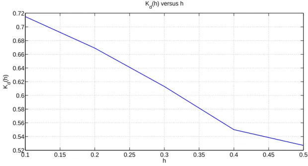
0.1 0.15 0.2 0.25 0.3 0.35 0.4 0.45 0.5 0.5 1 1.5 2 2.5 3 3.5 4 4.5 5 K_d(h) versus h h K d (h)

(78)

0.1 0.15 0.2 0.25 0.3 0.35 0.4 0.45 0.5 0.4 0.6 0.8 1 1.2 1.4 1.6 1.8 2 K p(h) versus h h K p (h)

design method-I. 0.1 0.15 0.2 0.25 0.3 0.35 0.4 0.45 0.5 0.35 0.4 0.45 0.5 0.55 0.6 0.65 0.7 0.75 0.8 K d(h) versus h h K d (h)

(79)

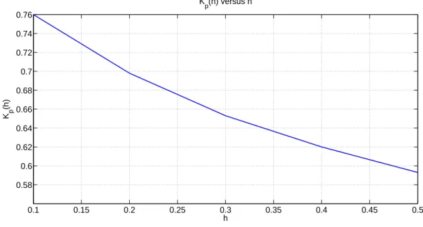
0.1 0.15 0.2 0.25 0.3 0.35 0.4 0.45 0.5 0.45 0.5 0.55 0.6 0.65 0.7 0.75 0.8 0.85 0.9 K p(h) versus h h K p (h)

design method-III.

From Table 3.4, again it can be concluded that as h increases, the upper limits for Kp for design method-I and design method-II become closer to each other and

become nearly the same at h = 0.5 sec. The lower limits for Kp are equal to each

other in two design methods and do not change with different h values, zero is the value of the unstable pole of P3(s).

When Table 3.5 is considered, it can be seen that as h increases, again Kd

and Kp values in both methods decrease. In addition, Kp values in each design

method become closer to each other as h increases.

If we compare Table 3.3 and 3.5, it can be concluded that as h increases, obtained PD controllers of P2(s) in each method becomes significantly equal to

(80)

3.4.4 Obtained PD Controllers and Allowable K

p

Ranges

for P

4

(s)

For each h value, the ranges for allowable Kp for P4(s) which are found by design

method-I and design method-II are listed in Table 3.6. Also, for each h value, least fragile PD controllers which are found by design method-I, gain margin optimizing PD controllers which are found by design method-II and least fragile PD controllers which are found by design method-III for P4(s) are listed in Table

3.7.

Design Method-I Design Method-II h = 0.1 0.001 < Kp < 2.89 0.001 < Kp < 1.019

h = 0.2 0.001 < Kp < 1.65 0.001 < Kp < 0.896

h = 0.3 0.001 < Kp < 1.24 0.001 < Kp < 0.806

h = 0.4 0.001 < Kp < 1.03 0.001 < Kp < 0.739

h = 0.5 0.001 < Kp < 0.91 0.001 < Kp < 0.685

Design Method-I Design Method-II Design Method-III h = 0.1 4.70s + 1.44 0.038s + 0.041 0.775s + 0.824 h = 0.2 2.25s + 0.83 0.033s + 0.037 0.601s + 0.668 h = 0.3 1.43s + 0.62 0.03s + 0.034 0.502s + 0.570 h = 0.4 1.04s + 0.51 0.027s + 0.032 0.428s + 0.503 h = 0.5 0.79s + 0.45 0.024s + 0.030 0.362s + 0.453

(81)

0.1 0.15 0.2 0.25 0.3 0.35 0.4 0.45 0.5 0.5 1 1.5 2 2.5 3 3.5 4 4.5 5 K d(h) versus h h K d (h)

design method-I. 0.1 0.15 0.2 0.25 0.3 0.35 0.4 0.45 0.5 0.4 0.6 0.8 1 1.2 1.4 1.6 1.8 2 K p(h) versus h h K p (h)

(82)

0.1 0.15 0.2 0.25 0.3 0.35 0.4 0.45 0.5 0.024 0.026 0.028 0.03 0.032 0.034 0.036 0.038 K d(h) versus h h K d (h)

design method-II. 0.1 0.15 0.2 0.25 0.3 0.35 0.4 0.45 0.5 0.03 0.032 0.034 0.036 0.038 0.04 0.042 K p(h) versus h h K p (h)

(83)

0.1 0.15 0.2 0.25 0.3 0.35 0.4 0.45 0.5 0.35 0.4 0.45 0.5 0.55 0.6 0.65 0.7 0.75 0.8 K d(h) versus h h K d (h)

design method-III. 0.1 0.15 0.2 0.25 0.3 0.35 0.4 0.45 0.5 0.58 0.6 0.62 0.64 0.66 0.68 0.7 0.72 0.74 0.76 K p(h) versus h h K p (h)

(84)

the upper limits for Kp for design method-I and design method-II become closer

to each other. The lower limits for Kp are equal to each other in two design

methods and do not change with different h values, 0.001 is the value of the unstable pole of P4(s).

When Table 3.7 is considered, it can be seen that as h increases, Kd and

Kp values in all methods decrease. In addition, Kp values in design method-I

and design method-III become closer to each other as h increases. Kd values

also become closer but not as significant as Kp values. Design method-II has

significantly small PD controller parameters compared to other methods because the unstable pole of P4(s) is very close to 0.

(85)

Chapter 4 TIME DOMAIN SIMULATIONS

AND ROBUSTNESS RESULTS

4.1 Robust Performance Test Results with

Ob-tained PD Controllers

It is known that the controller achieves robust performance if: (i) The nominal feedback system (C, P ) is stable, and

(ii) | W1(jw)S(jw) | + | W2(jw)T (jw) |≤ 1 for all w where W1(s) is the

performance weight, W2(s) is the robustness weight, S(s) = (1 + P (s)C(s))−1

is the sensitivity function and T (s) = 1 − S(s) is the complementary sensitivity function.

According to [23], any stabilizing C satisfies the robust performance condition for some specially defined weights W1(s) and W2(s). In practice, W1(s) and W2(s)

can be selected according to desire of assigning more weight to performance which means larger W1(s) and smaller W2(s) or assigning more weight to robustness

(86)

We want to investigate robust performance result of each PD controller derived for each plant. It is already known that first step for robust performance is satisfied as found controllers stabilize the plants. For the second condition, the inequality is modified as:

ρ | W1(jw)S(jw) | +k | W2(jw)T (jw) |≤ 1

and W1(s) and W2(s) are selected as:

W1 =

0.01 s W2 = 0.01s.

The reason for adding ρ and k to the inequality is that their values are going to show the performance quality of each feedback system. For each (C,P ) the largest ρ (ρmax) is found when k = 1. After that, the largest k (kmax) is found

when ρ = 1. Obtained ρmax and kmax values for P1(s), P3(s) and P4(s) are

compared for each delay and design methods. As P2(s) and PD controllers don’t

have a pole at s = 0, the robust performance test does not applied to P2(s) in

this thesis.

4.1.1 Robust Performance Test Results for P

1

(s)

For each h, obtained ρmax and kmax values for P1(s) are listed in Table 4.1. These

values are found from the least fragile PD controllers of P1(s) which are obtained

(87)

ρmax kmax h = 0.1 123 2.1 h = 0.2 81 4.0 h = 0.3 55 5.9 h = 0.4 40 7.7 h = 0.5 28 8.6

Table 4.1: Robust Performance Test Results for P1(s) with PD Controllers

Ob-tained from Design Method-I

Maximum | W1S | values as h increases are 0.0043, 0.0093, 0.0150, 0.0215

and 0.0309, respectively. In addition, maximum | W2T | values as h increases

are 0.4712, 0.2439, 0.1651, 0.1266 and 0.1121, respectively. As can be easily seen, maximum values of | W1S | and | W2T | do not have a linear increase and

decrease. So, the increase and decrease rate of maximum | W1S | and maximum

| W2T | affects the increase or decrease of ρmax and kmax. From Table 4.1, it can

be seen that ρmax decreases and kmax increases as h increases. When the increase

and decrease rates of maximum | W1S | and maximum | W2T | are considered,

this is an expected result.

4.1.2 Robust Performance Test Results for P

3

(s) and P

4

(s)

For each h, obtained ρmax and kmax values for P3(s) (also same for P4(s) as two

plants are almost equal) are listed in Table 4.2. These values are found from the least fragile PD controllers of P3(s) which are obtained from design method-I,

gain margin optimizing PD controllers of P4(s) which are obtained from design

method-II and least fragile PD controllers of P3(s) which are obtained from design

(88)

Design Method-I Design Method-II Design Method-III

ρmax kmax ρmax kmax ρmax kmax

h = 0.1 23 5 4.1 1600 44 38

h = 0.2 30 12 3.7 1800 46 43

h = 0.3 34 20 3.4 1900 41.8 54

h = 0.4 37 29 3.2 2100 41 62

h = 0.5 38 38 3 2300 40 85

Table 4.2: Robust Performance Test Results for P3(s) and P4(s)

For design method-I, maximum | W1S | values as h increases are 0.0349, 0.0302,

0.0276, 0.0261 and 0.0253 and maximum | W2T | values as h increases are 0.1818,

0.0786, 0.0473, 0.0333 and 0.0250, respectively. As both maximum | W1S | and

| W2T | decrease as h decreases, it is expected that ρmax and kmax increase

with the increase of h. From Table 4.2, it can be seen that expected results are obtained.

For design method-II, maximum | W1S | values as h increases are 0.2439,

0.2703, 0.2941, 0.3125 and 0.3333 and maximum | W2T | values as h increases

are 6.1 × 10−4, 5.4 × 10−4, 5 × 10−4, 4.6 × 10−4 and 4.2 × 10−4, respectively. Maximum | W1S | values increase but maximum | W2T | values decrease as h

increases. From Table 4.2, it can be seen that ρmax decreases and kmax increases

as h increases. When the increase and decrease rates of | W1S | and | W2T |

are considered, this is an expected result. Also, as maximum | W2T | values are

relatively very small, kmax values are expected to be relatively high which is also

an obtained result.

For design method-III, maximum | W1S | values as h increases are 0.0217,

0.0227, 0.0233, 0.0240 and 0.0247 and maximum | W2T | values as h increases are

0.0253, 0.0210, 0.0180, 0.0157 and 0.0138, respectively. When the increase and decrease rates of maximum | W1S | and | W2T | are considered, it is expected

(89)

When ρmax and kmax values for each design method are compared, it can be

concluded that best performance (largest ρmax), i.e., the best time tracking

per-formance is obtained with design method-III and best robustness (largest kmax)

(90)

4.2 Step Response Graphs for P

1

(s), P

3

(s) and

P

4

(s) with Obtained PD Controllers

In this section, step responses of P1(s), P3(s) and P4(s) are obtained for different h

values with PD controllers found by design methods. As P2(s) and PD controllers

do not have a pole at s = 0, it is expected that the step responses of P2(s) will

have a steady state error so the step responses of P2(s) are not included in the

thesis. On the other hand, P1(s), P3(s) and P4(s) have zero (or negligible errors)

steady-state errors as expected (due to a pole at s = 0 or nearby).

4.2.1 Step response Graphs for P

1

(s)

1. For h = 0.1 sec.

The step response of the feedback system with plant P1(s) and the controller

C(s) in (3.2) is obtained as: 0 0.5 1 1.5 2 2.5 3 3.5 0 0.5 1 1.5 2 2.5 Step Response Time (seconds) Amplitude

Figure 4.1: Step response of the feedback system with plant P1(s) and the

con-troller C(s) in (3.2) when h = 0.1 sec.

Design of PD controlleers for unstable infinitive dimensional plants with time-delay

DESIGN OF PD CONTROLLERS FOR

UNSTABLE INFINITE DIMENSIONAL

PLANTS WITH TIME-DELAY

a thesis submitted to

the graduate school of engineering and science

of bilkent university

in partial fulfillment of the requirements for

the degree of

master of science

in

electrical and electronics engineering

By

Deniz Varol

ABSTRACT

DESIGN OF PD CONTROLLERS FOR UNSTABLE

INFINITE DIMENSIONAL PLANTS WITH

TIME-DELAY

¨

OZET

KARARSIZ SONSUZ BOYUTLU VE ZAMAN

GEC˙IKMEL˙I MODELLER ˙IC

¸ ˙IN PD KONTROLC ¨

U

TASARIMI

Acknowledgement

Contents

List of Figures

List of Tables

Chapter 1

INTRODUCTION

1.1

Scope of the Thesis

1.2

Related Work

1.3

On PD Controllers

1.4

Organization of the Thesis

Chapter 2

PROBLEM DEFINITION

2.1

Feedback System Stability and Controller

Structure

2.2

Plant Types

Chapter 3

DESIGN OF PD

CONTROLLERS

3.1

Design Method-I: Design of Least Fragile

PD Controllers

3.1.1

Least Fragile PD Controllers for P

(s)

3.1.2

Least Fragile PD Controllers for P

(s)

3.1.3

Least Fragile PD Controllers for P

(s)

3.2

Design Method-II: Design of Gain Margin

Optimizing PD Controllers Given in [1]

3.2.1

Gain Margin Optimizing PD Controllers for P

(s)

3.2.2

Gain Margin Optimizing PD Controllers for P

(s)

3.2.3

Gain Margin Optimizing PD Controllers for P

(s)

3.3

Design Method-III: Design of a PD

Con-troller Minimizing Fragility in the

Propor-tional Gain Given in [1]

3.3.1

PD Controllers for Minimizing Fragility in the

Pro-portional Gain for P