The Taylor curve: international evidence

(1)

Full Terms & Conditions of access and use can be found at

https://www.tandfonline.com/action/journalInformation?journalCode=raec20

Applied Economics

ISSN: (Print) (Online) Journal homepage: https://www.tandfonline.com/loi/raec20

The Taylor curve: international evidence

Semih Emre Çekin, Rangan Gupta & Eric Olson

To cite this article: Semih Emre Çekin, Rangan Gupta & Eric Olson (2021): The Taylor curve: international evidence, Applied Economics, DOI: 10.1080/00036846.2021.1907284

To link to this article: https://doi.org/10.1080/00036846.2021.1907284

Published online: 11 Apr 2021.

Submit your article to this journal

Article views: 16

View related articles

(2)

The Taylor curve: international evidence

Semih Emre Çekina_{, Rangan Gupta} b _{and Eric Olson}c

a_{Department of Economics, Turkish-German University, Istanbul, Turkey;}b_{Department of Economics, University of Pretoria, Pretoria, South} Africa; c_{College of Business, University of Tulsa, Tulsa, Oklahoma, United States}

ABSTRACT

We use the Taylor curve to gauge deviations of monetary policy from an efficiency locus for the United Kingdom (UK) and the four largest economies of the Eurozone (Germany, France, Italy, Spain) for the period 2000–2018. For this purpose, we use shadow interest rates, which is a common metric for both conventional and unconventional monetary policies, and the newly proposed Hamilton-filter to measure output gap, which improves upon the drawbacks of the traditionally used Hodrick–Prescott filter. Our findings suggest that deviations in the UK mostly occurred amid the global financial crisis and the post-Brexit period, whereas Eurozone members experienced more volatile deviations around 2001, during the global financial crisis and the Eurozone sovereign debt crisis.

KEYWORDS

Taylor curve; monetary policy; eurozone; hp filter

JEL CLASSIFICATION

E31; E58; C32

I. Introduction

The efficacy of monetary policy implementation by central banks and its effect on the economy have received considerable interest in the macroeco-nomics literature. As part of this literature, a myriad of authors who analysed the recent mone-tary policy experience of the US, the United Kingdom (UK) and the Eurozone conclude that the substantial decrease in inflation levels and vola-tilities after the 1990s was – among other factors – due to effective monetary policy conduct.1 While inflation rates remained low throughout the 2000 decade in these economies, the post-2008 period brought new challenges for central banks. Faced with the zero-lower bound for nominal interest rates and a threat of deflation, central banks of most advanced economies engaged in unconven-tional policies. Most authors find that these policies had desirable effects, but an important question remains to be answered regarding the appropriate-ness of these policies and the extent to which they deviated from an optimal policy mix. One of the models that allows one to tackle this question is the Taylor curve, which was introduced by Taylor (1979) and relates second moments of output and inflation. As Friedman (2010) argues, this second-

order Phillips curve can be thought of as an effi-ciency locus through which one can gauge the appropriateness of monetary policy.

Previous works that used the Taylor curve to analyse the efficacy of monetary policy include Olson and Enders (2012) who analysed the case of the US, and Olson and Wohar (2016) who ana-lysed the case of the euro area and a set of European countries. While our methodology follows Taylor (1979) and is similar to the aforementioned works, our empirical strategy departs from these studies: we analyse the time period 2000–2018, i.e. the interval that encompasses the Great Recession and resulted in the zero-lower bound for most advanced economies. Correspondingly, we make use of the shadow interest rate measure of Wu and Xia (2016) to capture the stance of central banks when nominal interest rates are constrained by the zero lower bound. Another dimension in which our work departs from previous studies is the filtering methodology that we use in order to get a measure of the output gap. In all the above cited studies, the authors use the widely used Hodrick–Prescott (HP) filter (Hodrick & Prescott,

1997). However, Hamilton (2018) argues that the HP filter has important shortcomings that should prevent its use in empirical applications. In

CONTACT Eric Olson eric-olson@utulsa.edu College of Business, University of Tulsa, Tulsa, Oklahoma, United States

1

For authors who attribute the decline in inflation levels and volatilities to changes in the conduct of monetary policy, see among others Galí and Gambetti (2009) for the US, Batini and Nelson (2005) for the UK and Avouyi-Dovi and Sahuc (2016) for the euro area.

https://doi.org/10.1080/00036846.2021.1907284

(3)

analysing monetary policy efficacy, we utilize both filters and contrast them. We implement our esti-mation for five large European countries: UK, France, Germany, Italy and Spain.

First, our results indicate that the filtering meth-odology selected for the output gap produces sig-nificant differences in our monetary policy efficacy measures. Using the Hamilton filer, we find that – with the notable exception of France – monetary policy deviates from its optimum more signifi-cantly in the period after the Great Recession in comparison to the period preceding it. We deduce from these results that while most studies establish that the results of unconventional policies imple-mented by central banks had a desirable effect on distressed markets, they were not necessarily opti-mal. The paper is organized as follows: section 2

provides an overview of model, section 3 intro-duces the estimation strategy and data, section 4

the results and finally, section 5 concludes.

II. Methodology

The original Taylor curve begins with a central bank trying to minimize the expected value of the loss function (L): L ¼ λ πt π�t �₂ þð1 λÞ yt y�t �₂ (1) where πt is the inflation rate,π�t is the target

tion rate,λ is the central bank’s preference for infla-tion stability,yt is output, and y�t is the target level of

output. Consider the points and Taylor curve dis-played in Figure 1. Monetary policy that is optimal (that is, policymakers that chose an interest rate

path that minimized (1) subject to a structural model of the economy) would result in an economy functioning on, or near, its efficiency frontier such as point A. An interest rate path that was suboptimal would result in the observed volatilities being greater and would result in an economy operating to the right of the observed Taylor curve (for example, point B). As such, movement of the economy towards the Taylor curve would represent an improvement in the efficacy of mone-tary policy. Shifts in the Taylor curve itself, would result from technological changes in the structure of the economy that lowered the variability of the shocks that the economy undergoes. Likewise, the curvature of the Taylor curve of the efficiency fron-tier could change as well from technological changes which would alter the tradeoff between stabilizing inflation volatility in terms of output gap volatility.

We utilize a setup as in Cecchetti, Flores- Lagunes, and Krause (2006):

y¼_t X n i¼1 α1;i yt iþ Xn i¼1 β_1;i πt iþ Xn i¼1 ϕ_1;i it i þε1;t (2) π¼_t X n i¼1 α2;i yt iþ Xn i¼1 β_2;i πt iþ Xn i¼1 ϕ_2;i it i þε2;t (3)

where (2) is an aggregate demand function with the output gap yt depending on its own lags, lags of the inflation rate πt and lags of the nominal interest rate it. Similarly, equation (3) represents a Phillips

curve setup in which the inflation rate depends on lagged output gap, inflation and nominal interest rate terms. For the construction of Taylor curves, we follow the methodology as outlined in Taylor (1979) and Olson and Enders (2012) where the model that was introduced in (2) and (3) is

expressed in the following state-space

representation: Y¼_t BYt 1þcit 1þvt (4) with L ¼ λ πt π�t �₂ þð1 λÞ yt y�t �₂ (5) A B Output Volatility Inflation Volatility

(4)

The loss function in (1) is also rewritten as:

Y0tΛYt (6)

where Λ is an n × n weighting matrix with λ as the first diagonal element, (1-λ) as the nth diagonal element and the remaining elements equal to zero. Correspondingly, it is the central bank’s objective to choose the interest rate path that mini-mizes the loss function in (6) subject to (4) as the constraint. Given (6), the solution for the interest rate it is given as:

it ¼g Y_{t 1} (7)

Using optimal control techniques, the control vec-tor g is given by:

g ¼ ðc0HcÞ 1c0HB (8) with H representing the solution of the equations

H ¼ Λ þ ðB þ cgÞ0HðB þ cgÞ (9) Finally, with a set of feedback coefficients, g is expressed by (7), and the steady-state covariance

matrix of Yt is given by Σ:

� ¼Ω þ ðB þ cgÞ0�ðB þ cgÞ (10) where Ω is the covariance matrix of the residuals in

vt and the first and nth diagonal elements of

contain the steady-state variances. While one can determine a single point of the Taylor curve using a particular λ, varying λ over the interval [0,1] with steady state variances in results in the entire Taylor curve.

III. Estimation and data

We estimate the VAR setup in (2) and (3) with 120- month rolling windows, where n, the lag length for each VAR, was selected using the general-to- specific methodology. The Taylor curve was then

derived from an estimated VAR by implementing the procedure outlined previously, allowing n to change for each rolling window for each country that we consider.

To construct a relative distance measure that captures monetary policy efficacy while accounting for shifts in the Taylor curve, the minimum dis-tance at which a country operated from its Taylor curve for a specific 120 month window was calcu-lated, then divided by the minimum distance that the Taylor curve was from the origin for the same

120 month window.2

We estimate the Taylor curve for Great Britain, Germany, France, Italy and Spain using monthly data spanning January 1991–December 2018. Because we use a 120 month rolling window and our first sample encompasses the period 1991–2000, our Taylor curve estimates start in 2001. Consumer Price Index and industrial pro-duction series from the OECD main economic indicators database were used to calculate the infla-tion rate and output gap measures, respectively. IV. Shadow interest rates

The concept of shadow rates was introduced by Black (1995) in the modelling of the yield curve to account for negative rates. The relationship between the shadow rate and the nominal short- term interest rate is defined such that the short- term rate is the maximum of zero and the shadow interest rate. In other words, the shadow interest rate is equal to the short-term rate when it is positive but – in contrast to the short-term rate – it can also be negative. While the shadow interest rate was initially used in the modelling of the yield curves, recent studies used the concept to develop models that could circumvent the ZLB in the ana-lysis of quantitative easing measures and capture the stance of monetary policy. As alluded to in the

2_{We calculate two orthogonal distance measure in order to calculate our measures. That is, we first calculate the minimum distance between the observed}

volatilities and the efficiency frontier:

dmin¼ ffiffiffiffiffiffiffiffiffiffiffiffiffiffiffiffiffiffiffiffiffiffiffiffiffiffiffiffiffiffiffiffiffiffiffiffiffiffiffiffiffiffiffiffiffiffiffiffiffiffiffiffiffiffiffiffiffiffiffiffiffiffiffiffiffiffiffiffiffiffiffiffiffiffiffiffiffiffiffiffiffiffiffiffiffiffiffi σoptimalπ σobservedπ � �2 þ σoptimaly σobservedy � �2 r

We subsequently calculate the minimum distance between the efficiency frontier and the origin:

dmin1¼ ffiffiffiffiffiffiffiffiffiffiffiffiffiffiffiffiffiffiffiffiffiffiffiffiffiffiffiffiffiffiffiffiffiffiffiffiffiffiffiffiffiffiffiffiffiffiffiffiffiffiffiffiffiffiffiffiffiffiffiffiffiffiffi 0 σoptimalπ � �₂ þ 0 σoptimaly � �₂ r

and then divide dmin/dmin1. Because the efficiency frontier is in output volatility and inflation volatility space, the units are best thought of as combinations

(5)

introduction section, we use the shadow interest rate measure of Wu and Xia (2016, 2017) for the UK and Eurozone, which is estimated and derived from a three-factor shadow rate term structure model (SRTSM).3 Further, while for the UK the shadow interest rate measure was used for the entire period, for the remaining countries, the Eonia (Euro overnight index average) was used for the pre-2004 period and the shadow rate of

Wu and Xia (2016) was used for the

2004–2018 period.4

V. Output gap estimates

Output gap estimates are typically estimated using two approaches: the statistical filtering approach (e.g. the Hodrick–Prescott filter) which specifies a statistical methodology to extract unobserved trends and cycles of a time series, and the structural approach which estimates the output gap using a structural model of the economy. For the estima-tion of the output gap in the present work, we use and contrast two widely used approaches, the HP filter, formulated by Hodrick and Prescott (1997) and the regression filter introduced by Hamilton (2018). Hamilton (2018) argues that the HP filter produces spurious cycles, exhibits an end-of- sample bias with filtered values at the end of the sample being very different from values in the middle, and that suggested values of the smoothing parameter lambda are not appropriate for the fil-tering procedure. He suggests an alternative filter that one can obtain by regressing a variable at date

t + h on its most recent four observations that

remedies these shortcomings. Studies that contrast the two filters argue that the Hamilton filter is superior to the HP filter, mostly because the latter exhibits a stronger end-of-sample bias (Schüler

2018; Jönsson 2019).

VI. Results

Tables 1 and table 2 display our monetary policy

efficacy measures. From Tables 1 and table 2 it is clearly visible that the two filtering methodologies

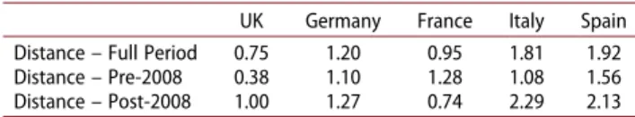
produce drastically different distance averages in quantitative terms. Specifically, the distance results that we obtained using the Hamilton filter are higher for all economies with the exception of Italy. Another important result is that the measures obtained by both filters imply that in the period after the financial crisis monetary policy efficacy deteriorated and distances increased for all coun-tries (except for France). Below, we further discuss the distance measures that we obtained using the Hamilton filter for the five economies we have considered.

Monetary policy efficacy UK

The recent monetary policy experience of the UK is shaped by the financial crisis of 2008 and the sub-sequent response of the Bank of England (BoE). In response to the financial crisis, the BoE did not initially engage in quantitative easing (QE) but took several measures such as the Special Liquidity Scheme (SLS) and Discount Window Facility after the collapse of Bear Stearns in April 2008. The stance of monetary policy changed significantly only after 2008, when interest rates were decreased after the events of September 2008 and wide-ranging QE measures were introduced after March 2009 with the Asset Purchase Facility (APF) and the gilt purchase programme (see Joyce, Tong, and Woods 2011 for an account of the mea-sures taken by the BoE after 2008).

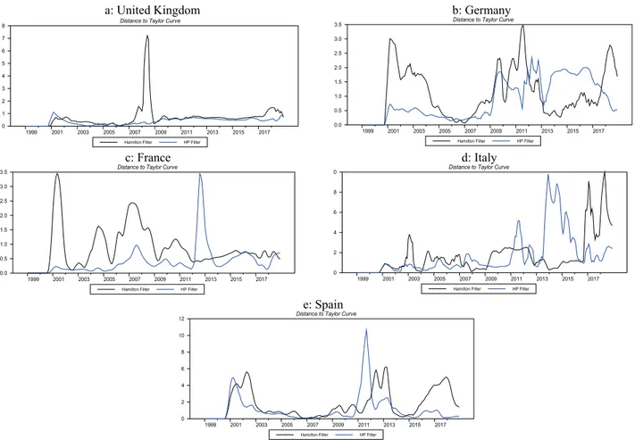
Corresponding to these developments, our esti-mates (Figure 2a) imply that the use of both filters

Table 1. Distance measures obtained using the Hamilton Filter.

UK Germany France Italy Spain

Distance – Full Period 0.75 1.20 0.95 1.81 1.92

Distance – Pre-2008 0.38 1.10 1.28 1.08 1.56

Distance – Post-2008 1.00 1.27 0.74 2.29 2.13

Table 2. Distance measures obtained using the HP Filter.

Distance – Full Period 0.42 0.97 0.45 1.82 1.21

Distance – Pre-2008 0.25 0.36 0.25 0.67 1.06

Distance – Post-2008 0.52 1.37 0.58 2.57 1.31

3_{The data is available for download from the website of Professor Jing Cynthia Wu at:}_{https://sites.google.com/view/jingcynthiawu/shadow-rates?authuser=0}_. 4

The shadow rate for the Eurozone is available for the period after 2004. Because shadow rates and nominal interest rates exhibit minimal discrepancy before the 2008 period, i.e. during the period when shadow rates are not negative, this approach does not pose a methodological challenge. Table A1 displays the summary statistics for the variables used in the analysis.

(6)

delivers very similar Taylor curve distance esti-mates with two exceptions: (1) in the 2007–2009 period, the use of the HP filter does not generate any significant deviation from the Taylor curve for the period. In contrast to this, use of the Hamilton filter results in a very signifi-cant spike, suggesting that monetary policy deviated from its optimum during the Great Recession. However, this deviation is short lasted and the distance to the Taylor curve reverts back to the pre-financial crisis period. (2) The distance measure that we obtain using the Hamilton filter increases once more after 2017 while using the HP filter doesn’t result in a discernible change. These results are in line with the recent monetary policy experience of the UK. Notably, the benchmark interest rate was raised by the Bank of England until July 2007 and remained high until the collapse of Lehman Brothers in September 2008, while the output gap (obtained with the Hamilton filter) shows a significant drop after February 2008. Likely due to this mismatch, there is a significant

increase in the distance measure during the period March 2008–September 2008. Prior to the slight increase of the distance measure at the end of 2017, events such as the Brexit vote and a decision by the BoE to raise interest rates occurred while the output gap measure implied that the economy operated above its potential level. ECB policies

The ECB started its operations in 1999, having been established with the aim to conduct monetary policy for all Eurozone members. While in its first few years the ECB conducted its operations in relative peace, it faced significant challenges in later years, especially with the onset of the financial crisis in 2008 and Eurozone sovereign debt crisis after 2010. The pri-mary response of the ECB to the 2008 crisis, to lower interest rates, was quickly faced with the zero lower bound (ZLB) by the end of 2009. In response to reaching the ZLB, the ECB implemented several unconventional measures and quantitative easing policies that were similar to the measures taken by

a: United Kingdom b: Germany

c: France d: Italy

e: Spain United Kingdom

Distance to Taylor Curve

Hamilton Filter HP Filter

1999 2001 2003 2005 2007 2009 2011 2013 2015 2017 0 1 2 3 4 5 6 7 8 Germany

1999 2001 2003 2005 2007 2009 2011 2013 2015 2017 0.0 0.5 1.0 1.5 2.0 2.5 3.0 3.5 France

1999 2001 2003 2005 2007 2009 2011 2013 2015 2017 0.0 0.5 1.0 1.5 2.0 2.5 3.0 3.5 Italy

1999 2001 2003 2005 2007 2009 2011 2013 2015 2017 0 2 4 6 8 10 Spain

1999 2001 2003 2005 2007 2009 2011 2013 2015 2017 0 2 4 6 8 10 12

(7)

the Federal Reserve. Of these, the most relevant programmes included the ‘Securities Markets Programme’ (SMP) I and II of 2011, ‘Outright Monetary Transactions’ (OMT) of 2012 and the ‘Asset Purchase Programme’ (APP) of 2015 (see e.g. Fratzscher, Duca, and Straub 2016 for a description of unconventional policies that the ECB implemented after 2008). As summarized in Dell’Ariccia, Rabanal, and Sandri (2018), studies that analyse the effect of unconventional policies implemented by the ECB on Eurozone members mostly find that the measures positively affected bond yields, output growth and prices. Despite these results, some of the policies may have been inappropriate for individual members as a consequence of the fact that the ECB conducts policy for the Eurozone as a whole and not for the needs of individual members as argued in Moons and Van Poeck (2008). In the following, we will describe our results for a set of Eurozone countries and analyse how policy may have deviated from its optimum for these countries.

Germany

The distance estimates for Germany differ signifi-cantly with the use of the two filters (Figure 2b): according to the HP filter, there is significant devia-tion of monetary policy from its optimum after the Great Recession, and another increase after 2013. In contrast, the Hamilton filter shows a significant spike after 2001, which gradually decreases until the Great Recession. During this period, the output gap increased and remained high until the first months of 2008 while interest rates remained steadily high. With the onset of the Great Recession, there was a sharp drop in the output gap while the interest rate decreased gradually. During this time, the dis-tance increases significantly and remains high until the end of 2012. This is the time when the ECB implemented many of the unconventional quantita-tive easing measures to combat the effects of the Eurozone sovereign debt crisis that engulfed coun-tries such as Greece, Spain, Portugal and Ireland. Finally, the distance increases once more after June 2017 when the output gap increases significantly, while the shadow interest rate goes further into nega-tive territory.

France

For France, our results suggest once more that the two filters produce very different Taylor curves (Figure 2c). The distance to the Taylor curve that is based on the HP filter increases in 2007 and in 2012 while remaining relatively low during the remaining peri-ods. In contrast to this, the magnitude of the distance measure that is based on the Hamilton filter is higher on average and increases during several periods. In 2001, the distance is at its highest level and coincides with a high output gap and decreasing interest rates. In 2004, the distance reaches elevated levels when output gap fluctuated, and the shadow interest rate remained relatively high. Similarly, the distance increases and remains relatively high between 2006 and 2009 when interest rates remain on an increasing trend while the output gap fluctuates between the 2–5% band. Finally, the distance increases only slightly after the outbreak of the financial crisis but remains low for the remaining observation period. It is interesting to see that the distance measure for France is lower on average in comparison to the distance measures of other Eurozone economies under consideration and doesn’t exhibit significantly elevated levels during the aftermath of the financial crisis or the Eurozone crisis. This may indicate that the measures taken by the ECB were in line with monetary policy requirements of the French economy.

Italy

In Italy’s case, the two distance measures move in relative tandem until 2009, after which significant differences appear (Figure 2d): with the HP filter, the distance increases in 2011 and between 2013 and 2016, whereas with the Hamilton filter, dis-tance to the Taylor curve remains high between 2009 and 2013 and after 2016. The first significant increase of the distance during 2009–2013 coin-cides with the aftermath of the financial crisis and with the Eurozone crisis which engulfed Italian bond markets and increased the cost of lending through sovereign spread movements (Albertazzi et al. 2014). As outlined above, the ECB implemen-ted a number of unconventional measures to com-bat the turmoil in financial markets and authors such as Casiraghi et al. (2016) find that these

(8)

measures had a significant and positive effect on Italy’s economy in 2011–2012. During this period, the distance measure increases which is likely due to the output gap estimate becoming negative while the shadow interest rate increased periodically. Only after 2012, the interest rate decreases again, notably after the ‘Whatever it takes’ speech by for-mer ECB President Mario Draghi in July 2012 and details of the Outright Monetary Purchase (OMT) measure were shared with the public in September 2012. Similarly, the drastic increase of the distance measure after October 2016 coincides with the first significant increase of the output gap after 2008 while the shadow interest rate decreased further into negative territory. It is likely due to this mismatch that the distance measure reaches its highest level during our estimation period.

Spain

The two distance measures for Spain also move in relative tandem until 2011 (Figure 2d). After this period, use of the HP filter produces a significant increase in the distance between mid-2010 to mid 2012, whereas with the use of the Hamilton filter, the distance increases for the periods 2001–2003, 2011–2013 and 2015–2018. During the first spike of 2001–2003, Spain was in the course of imple-menting a series of stability measures to comply with fiscal policy requirements set by the EU. While these policies proved successful5 and the output gap was relatively high, the ECB policy rate was continuously decreased during this time. Interestingly, the distance measure remained rela-tively low during the financial crisis, but increased substantially after 2011 when the Eurozone crisis encompassed Spain and other member economies. The crisis affected Spain significantly when bond premiums reached high levels in mid-2012 and the output gap decreased. At the same time, the inter-est rate was decreased until mid-2012 but then slightly increased until the end of 2013, likely caus-ing the mismatch that led to an increase in the distance measure. As referred to above, the ECB implemented a myriad of unconventional mea-sures to support financial markets in the Eurozone area, causing (shadow) interest rates to go further into the negative territory after 2013. Of

these, the most significant announcement was the large asset purchasing programme after 2015. Against this background, countries such as Spain recovered from the effects of the Eurozone crisis and recorded falling bond premiums and positive output gaps after 2015. During this time, the dis-tance measure increases once more and remains high until the end of 2018.

Discussion

A number of studies analysed the optimality of monetary policy using policy rules or DSGE mod-els and established that while central banks’ aggres-sive stance towards inflation lowered inflation rates after the 1980s in most advanced economies, they were not necessarily optimal. For example, Chen and MacDonald (2012) show that monetary policy in the UK was suboptimal in comparison to an optimized policy rule. Similarly, Benigno and Lopez-Salido (2006) show that over the period 1970–1997 monetary policy in a set of euro area economies was not always optimal in terms of welfare considerations.

Our results are mostly supportive of the view presented in these works that monetary policy underwent periods that deviated from an efficiency locus. But while these works don’t necessarily inform the reader about the degree to which policy deviated from the optimum over time, our results give us an insight into the timing and severity of deviations from the optimum. Specifically, we find that for most of the Eurozone member countries we consider (Germany, France, Spain) there is a significant deviation from the optimum at around 2001. This is likely due to the fact that in the first few years after the Eurozone was established, infla-tion differentials were especially wide among mem-ber economies (see e.g. Lane 2006 for this point). While inflation rates converged in subsequent years, the post-2008 period that included the global financial crisis and the Eurozone crisis associated with sovereign debt affected all countries to various extents. Not surprisingly, the 2008–2012 and the post-2015 periods are shaped by significant devia-tions from the efficiency locus for these economies, implying that the policies that the ECB

5

(9)

implemented were not optimal. As a notable excep-tion, our results indicate that monetary policy in France deviated from the optimum around 2001 and during the period 2004–2009, while staying close to the optimum after 2011. The most likely explanation is that France’s output gap was the least volatile among the Eurozone members that we consider, and its inflation volatility was the second lowest (after Germany).

These results are in line with recent evidence regarding the appropriateness of the single mone-tary policy regime of the ECB for individual mem-ber economies. For example, Fries et al. (2018) find that the effect of the regime was almost neutral for France in the post global financial crisis period while for Spain, it was too accommodative in the first half of the 2000 decade and too restrictive during the crisis years of 2011–2013. Finally, UK stands out in our analysis as the economy with the lowest overall distance to the efficiency locus. This is likely a reflection of the fact that the UK is not a member of the Eurozone and was able to imple-ment more targeted monetary policy measures in response to movements in the output gap and inflation rates.

VII. Conclusion

In this work, we analysed monetary policy efficacy for the UK and four largest economies of the Eurozone using the Taylor curve for the period 2000–2018. While our approach is not novel, our empirical implementation makes use of shadow interest rates and a new output gap measure, both of which were developed recently. Our findings suggest that UK’s monetary policy deviated signifi-cantly around during the global financial crisis but remains close to the efficiency locus for the remain-ing period. In contrast to this, with the exception of France, whose deviations from the efficiency locus remain relatively low, Eurozone members’ mone-tary policy deviated significantly around 2001, dur-ing the global financial crisis and durdur-ing the Eurozone crisis. The implications of our results are manifold. We find that the ECB’s single policy regime likely resulted in deviations of individual members’ policies from an efficiency locus,

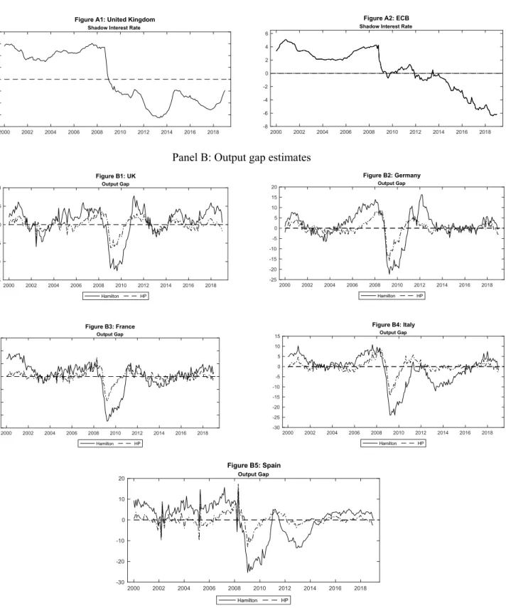
supporting previous studies (e.g. Fries et al. 2018) while the UK experienced deviations only for a brief period. This highlights the difficulties of conducting monetary policy for economies with differing output gaps and inflation differentials and calls for coordinated policies by individual member countries to complement the policies of the ECB. Our results also have implications on the methodological choice: previous studies such as Olson and Wohar (2016) used overnight rates and the HP Filter to gauge the efficacy of monetary policy using the Taylor curve. Because our sample encompasses the post-2008 period, we used the shadow rate of Wu and Xia (2016) for the stance of monetary policy and used the Moons and Van Poeck (2008) to model the output gap. As a consequence of our methodological choice, the Hamilton filter suggests that movements in the output gap were more pronounced in comparison to the HP filter for all countries we consider, and the shadow interest rate suggests that the stance of monetary policy in the UK and in the Eurozone was more accommodative than what is implied by the use of overnight interest rates (Figures A1–A8). The differences between our study and previous studies are likely to have a significant effect on the estimation outcome: Olson and Wohar (2016) find that for France, Germany, Italy and Spain the dis-tance measure increased similarly and mainly after the onset of the 2008 crisis and stayed high for the remainder of the analysis. In contrast, we find that in France monetary policy deviated more from its efficiency locus before the 2008 period than it did after the 2008 period. We also find that monetary policy deviated from its efficiency locus more sig-nificantly in the post-2008 period in Italy and Spain, suggesting that ECB policy during this per-iod was more accommodating for larger econo-mies. The latter finding supports the finding of Crowley and Lee (2009) that ECB policy is gener-ally more accommodating for Germany and France.

Considering these findings, we believe that our results provide a more nuanced picture of events and highlight the relevance of using appropriate measures for modelling the stance and appropri-ateness of monetary policy.

(10)

Disclosure statement

No potential conflict of interest was reported by the authors.

ORCID

Rangan Gupta http://orcid.org/0000-0001-5002-3428

References

Albertazzi, U., T. Ropele, G. Sene, and F. M. Signoretti. 2014. “The Impact of the Sovereign Debt Crisis on the Activity of Italian Banks.” Journal of Banking & Finance 46: 387–402. doi:10.1016/j.jbankfin.2014.05.005.

Avouyi-Dovi, S., and J. G. Sahuc. 2016. “On the Sources of Macroeconomic Stability in the Euro Area.” European

Economic Review 83: 40–63. doi:10.1016/j. euroecorev.2015.11.012.

Batini, N., and E. Nelson (2005). “The UK’s Rocky Road to Stability”. FRB of St. Louis Working Paper 2005–2020.

Benigno, P., and J. D. Lopez-Salido. 2006. “Inflation Persistence and Optimal Monetary Policy in the Euro Area.” Journal of Money, Credit, and Banking 38 (3): 587–614. doi:10.1353/mcb.2006.0038.

Black, F. 1995. “Interest Rates as Options.” The Journal of Finance 50 (5): 1371–1376. doi:10.1111/j.1540-6261.1995.tb05182.x. Casiraghi, M., E. Gaiotti, L. Rodano, and A. Secchi. 2016.

“ECB Unconventional Monetary Policy and the Italian Economy during the Sovereign Debt Crisis.”

International Journal of Central Banking 12 (2): 269–315.

Cecchetti, S. G., A. Flores-Lagunes, and S. Krause. 2006. “Has Monetary Policy Become More Efficient? A Cross-Country Analysis.” The Economic Journal 116 (511): 408–433. doi:10.1111/j.1468-0297.2006.01086.x.

Chen, X., and R. MacDonald. 2012. “Realized and Optimal Monetary Policy Rules in an Estimated Markov-Switching DSGE Model of the United Kingdom.” Journal of Money,

Credit, and Banking 44 (6): 1091–1116. doi:10.1111/j.1538- 4616.2012.00524.x.

Crowley, P. M., and J. Lee (2009). “Evaluating the Stresses from ECB Monetary Policy in the Euro Area”. Bank of Finland Research Discussion Paper, (11).

Dell’Ariccia, G., P. Rabanal, and D. Sandri. 2018. “Unconventional Monetary Policies in the Euro Area, Japan, and the United Kingdom.” Journal of Economic

Perspectives 32 (4): 147–172. doi:10.1257/jep.32.4.147. Fratzscher, M., M. L. Duca, and R. Straub. 2016. “ECB

Unconventional Monetary Policy: Market Impact and International Spillovers.” IMF Economic Review 64 (1): 36–74. doi:10.1057/imfer.2016.5.

Friedman, M. 2010. “Trade-offs in Monetary Policy.” In: Robert Leeson (ed) David Laidler’s Contributions to

Economics, 114–127. London: Palgrave Macmillan.

Fries, S., J. S. Mésonnier, S. Mouabbi, and J. P. Renne. 2018. “National Natural Rates of Interest and the Single Monetary Policy in the Euro Area.” Journal of Applied

Econometrics 33 (6): 763–779. doi:10.1002/jae.2637. Galí, J., and L. Gambetti. 2009. “On the Sources of the Great

Moderation.” American Economic Journal:

Macroeconomics 1 (1): 26–57.

Hamilton, J. D. 2018. “Why You Should Never Use the Hodrick-Prescott Filter.” Review of Economics and

Statistics 100 (5): 831–843. doi:10.1162/rest_a_00706. Hodrick, R. J., and E. C. Prescott. 1997. “Postwar U.S.

Business Cycles: An Empirical Investigation.” Journal of

Money, Credit, and Banking 29 (1): 1–16. doi:10.2307/ 2953682.

Jönsson, K. 2019. “Real-time US GDP Gap Properties Using Hamilton’s Regression-based Filter.” Empirical Economics59: 1–8.

Joyce, M., M. Tong, and R. Woods. 2011. “The United Kingdom’s Quantitative Easing Policy: Design, Operation and Impact.” Bank of England Quarterly Bulletin. Q3. Lane, P. R. 2006. “The Real Effects of European Monetary

Union.” Journal of Economic Perspectives 20 (4): 47–66. doi:10.1257/jep.20.4.47.

Moons, C., and A. Van Poeck. 2008. “Does One Size Fit All? A Taylor-rule Based Analysis of Monetary Policy for Current and Future EMU Members.” Applied Economics 40 (2): 193–199. doi:10.1080/00036840600749763.

OECD (Organisation for Economic Co-operation and Development) (2001a), “OECD Economic Surveys: Spain 2001”, OECD Publishing, Paris.

Olson, E., and W. Enders. 2012. “A Historical Analysis of the Taylor Curve.” Journal of Money, Credit, and Banking 44 (7): 1285–1299. doi:10.1111/j.1538-4616.2012.00532.x. Olson, E., and M. E. Wohar. 2016. “An Evaluation of ECB

Policy in the Euro’s Big Four.” Journal of Macroeconomics 48: 203–213. doi:10.1016/j.jmacro.2016.03.001.

Schüler, Y. S. (2018). “On the Cyclical Properties of Hamilton’s Regression Filter”. Deutsche Bundesbank Discussion Paper No. 03/2018.

Taylor, J. B. 1979. “Estimation and Control of a Macroeconomic Model with Rational Expectations.”

Econometrica: Journal of the Econometric Society 47 (5):

1267–1286. doi:10.2307/1911962.

Wu, J. C., and F. D. Xia. 2016. “Measuring the Macroeconomic Impact of Monetary Policy at the Zero Lower Bound.”

Journal of Money, Credit, and Banking 48 (2–3): 253–291.

doi:10.1111/jmcb.12300.

Wu, J. C., and F. D. Xia (2017). “Time-varying Lower Bound of Interest Rates in Europe”. Chicago Booth Research Paper, (06–17).

(11)

Appendix A

Table A1. Summary statistics of key indicators

Panel A. Shadow interest rates for the UK and ECB.

Panel A: Shadow interest rates for the UK and ECB

Panel B: Output gap estimates 2000 2002 2004 2006 2008 2010 2012 2014 2016 2018 -8 -6 -4 -2 0 2 4 6 8

Figure A1: United Kingdom

Shadow Interest Rate

2000 2002 2004 2006 2008 2010 2012 2014 2016 2018 -8 -6 -4 -2 0 2 4 6

Figure A2: ECB

Shadow Interest Rate

2000 2002 2004 2006 2008 2010 2012 2014 2016 2018 -15 -10 -5 0 5 10 Figure B1: UK Output Gap Hamilton HP 2000 2002 2004 2006 2008 2010 2012 2014 2016 2018 -25 -20 -15 -10 -5 0 5 10 15 20 Figure B2: Germany Output Gap Hamilton HP 2000 2002 2004 2006 2008 2010 2012 2014 2016 2018 -20 -15 -10 -5 0 5 10 15 Figure B3: France Output Gap Hamilton HP 2000 2002 2004 2006 2008 2010 2012 2014 2016 2018 -30 -25 -20 -15 -10 -5 0 5 10 15 Figure B4: Italy Output Gap Hamilton HP 2000 2002 2004 2006 2008 2010 2012 2014 2016 2018 -30 -20 -10 0 10 20 Figure B5: Spain Output Gap Hamilton HP

(12)

Panel B. Output gap estimates.

Panel C: Key variables

2000 2002 2004 2006 2008 2010 2012 2014 2016 2018 -2 0 2 4 6 Figure C1: UK Key variables

10 year yield Inflation Real Int. Rate

2000 2002 2004 2006 2008 2010 2012 2014 2016 2018 -2 0 2 4 6 Figure C2: Germany Key variables

2000 2002 2004 2006 2008 2010 2012 2014 2016 2018 -2 0 2 4 6 Figure C3: France Key variables

2000 2002 2004 2006 2008 2010 2012 2014 2016 2018 0 2 4 6 8 Figure C4: Italy Key variables

2000 2002 2004 2006 2008 2010 2012 2014 2016 2018 -2 0 2 4 6 8 Figure C5: Spain Key variables

(13)

Panel C. Key variables.

Averages and standard deviations – 2000-2019

10 year bond yield 4.81

(0.37) 4.29 (0.62) 4.37 (0.65) 4.56 (0.65) 4.41 (0.71) Inflation rate 1.62 (0.50) 3.23 (0.60) 2.32 (0.38) 1.74 (0.52) 1.80 (0.39)

Real interest rate 2.67

(0.77) 1.18 (0.90) 2.23 (0.56) 3.07 (0.73) 2.57 (0.78)

Averages and standard deviations – 2000-2019

(1.10) 1.65 (1.29) 2.15 (1.29) 3.55 (1.44) 3.39 (1.63) Inflation rate 1.35 (0.80) 1.40 (1.61) 1.39 (1.20) 2.22 (1.04) 1.18 (0.96)

(1.28) 1.98 (1.60) 2.17 (0.87) 0.31 (1.13) 0.97 (1.18) Averages and standard deviations – 2000-2019

(1.42) 2.58 (1.68) 3.08 (1.53) 3.98 (1.28) 3.82 (1.42) Inflation rate 1.46 (0.70) 2.17 (1.57) 1.78 (1.05) 2.02 (0.89) 1.44 (0.83)

(1.60) 1.64 (1.41) 2.19 (0.75) 1.47 (1.68) 1.64 (1.30)