The impact of implicit government guarantees to sifis

i

T.C.

TURKISH-GERMAN UNIVERSITY

INSTITUTE OF SOCIAL SCIENCES

INTERNATIONAL FINANCE DEPARTMENT

THE IMPACT OF IMPLICIT GOVERNMENT

GUARANTEES TO SIFIS

MASTER’S THESIS

Burak SELÇOK

ii

T.C.

TURKISH-GERMAN UNIVERSITY

INSTITUTE OF SOCIAL SCIENCES

INTERNATIONAL FINANCE DEPARTMENT

THE IMPACT OF IMPLICIT GOVERNMENT

GUARANTEES TO SIFIS

MASTER’S THESIS

Burak SELÇOK

ADVISOR

Asst. Prof. Dr. Levent YILMAZ

iii

ACKNOWLEDGEMENT

I am grateful to my supervisor, Levent Yılmaz, for supporting me with guidance and helpful advice for this thesis.

I would like to also express my deepest gratitude to my wife, Ebru Aksu Selçok, for her patience and tolerance, I could not be able to finish this work without her support.

iv

TABLE OF CONTENTS

ENGLISH ABSTRACT ... vii

LIST OF ABBREVIATIONS... viii

LIST OF TABLES ... ix

1. INTRODUCTION ... 1

2. DEFINITIONS ... 3

2.1. CREDIT RATING AGENCIES AND CREDIT RATINGS ... 3

2.2. ORIGIN OF CREDIT RATING AGENCIES ... 4

2.3. THE BIG THREE CREDIT RATING AGENCIES ... 4

2.4. CREDIT RATING PROCESS AND SCALES ... 5

2.5. SYSTEMIC RISK ... 7

2.6. TOO BIG TO FAIL AND SYSTEMICALLY IMPORTANT FINANCIAL INSTITUTIONS ... 9

3. LITERATURE REVIEW ... 11

4. DATA DESCRIPTION ... 13

4.1. REFERENCE CREDIT RATINGS ... 13

4.1.1. Sovereign Long-Term Rating ... 13

4.1.2. Issuer Long-Term Ratings ... 13

4.1.3. Support Rating... 14

4.1.4. Support Rating Floor ... 15

4.1.5. Viability Rating ... 15

4.2. COLLECTED DATA ... 16

5. DESCRIPTIVE STATISTICS ... 18

5.1. REGRESSION ANALYSIS ... 20

5.2. ROBUSTNESS CHECKS VIA DUMMY VARIABLES ... 24

5.3. ROBUSTNESS CHECKS VIA SUBGROUPS ... 26

5.4. OTHER ROBUSTNESS CHECK ... 29

v

6.1. COMBINING RESULTS ... 31

6.2. CONCLUSION ... 34

REFERENCES ... 35

vi

TURKISH ABSTRACT

THE IMPACT OF IMPLICIT GOVERNMENT

GUARANTEES TO SIFIS

2008 küresel finans krizi sonrasında ortaya çıkan finansal kurum iflasları gösterdi ki devletler daha büyük bir ekonomik çöküşü engellemek amacıyla sistemik öneme sahip finansal kurumların iflas etmesine izin vermemektedir. Devletlerin bu kurumlara karşı olan bu tutumu yatırımcılar tarafından gizli bir garanti olarak algılanmakta olup bu gizli garanti sayesinde bu kurumlar bazı avantajlar elde etmektedir. Bu avantajların en önemlisi sistemik önemli bankaların fonlama maliyetlerinin sistemik öneme sahip olmayan finansal kurumlara kıyasla daha düşük olmasıdır. Bu çalışma ile söz konusu gizli garanti, finansal kurumların kredi derecelendirme notları aracığıyla sayısallaştırılmış olup 2019 yıl sonunda 22-30 baz puan aralığında bir maliyet avantajı sağlandığı görülmüştür.

Key Words: Sistemik Öneme Sahip Finansal Kurumlar, Banka Kurtarma, Sistemik Risk

vii

ENGLISH ABSTRACT

THE IMPACT OF IMPLICIT GOVERNMENT

GUARANTEES TO SIFIS

The financial institution bankruptcies that emerged after the 2008 global financial crisis showed that the governments do not allow Systemically Important Financial Institutions to bankrupt to prevent a more significant economic collapse. This attitude of governments towards these institutions is perceived as an implicit guarantee by investors, and thanks to this implicit guarantee, these institutions gain some advantages. The most important of these advantages is that the funding costs of Systemically Important Financial Institutions are lower compared to financial institutions that do not have systemic importance. With this study, this implicit guarantee has been quantified through the credit ratings of financial institutions, and it has been observed that a cost advantage was in the range of 22-30 basis points at the end of 2019.

Key Words: Systemically Important Financial Institutions, Bank Bailouts, Systemic Risk

viii

LIST OF ABBREVIATIONS

BIS : Bank for International Settlements

CR : Credit Ratings

CRA : Credit Rating Agencies

Fitch : Fitch Ratings

FSB : Financial Stability Board

ICBC : Industrial and Commercial Bank of China Limited

ILTR : Issuer Long Term Rating

IMF : International Monetary Fund

Moody’s : Moody’s Investors Service

OLS : Ordinary Least Square

OP : Ordered Probit Model

S&Ps : Standard & Poor's

SIFI : Systemically Important Financial Institutions

SLTR : Sovereign Long-Term Rating

SRF : The Support Rating Floors

SR : Support Ratings

TARP : Troubled Asset Relief Program

TBTF : Too Big To fail

USA : The United States of America

ix

LIST OF TABLES

PAGE NO

Table 1 : Number of Outstanding Credit Ratings as of

December 31, 2017 by Rating Category 5

Table 2 : Percentage by Rating Category of CRA as of

December 31, 2017 5

Table 3 : Credit Ratings Numerical Scale Correspondence 7

Table 4 : Distribution of the Sample by Country 17

Table 5 : Summary Statistics for Credit Ratings 18

Table 6 : Summary Statistic by Country Groups 18

Table 7 : Results of SR and Banks Asset Size Relationship 19

Table 8 : Results of Ordered Probit Regression 22

Table 9 : Credit Ratings of ICBC 23

Table 10 : Results of Ordered Probit Regression of 5 Subgroups 27

Table 11 : Results of OLS Regression 30

Table 12 : Summary of Regression Analysis 32

1

1. INTRODUCTION

This study aims to reveal and quantify the support provided by the governments to financial institutions because of their systemic importance. The government support has been analyzed through implicit government guarantees embedded in the credit ratings. It has been observed that as the systemic importance of a financial institution increases, the government guarantees increases. Therefore, to draw attention to the advantages of being systemically important, the title of the thesis was chosen as " The Impact Of Implicit Government Guarantees To Systemically Important Financial Institutions (SIFIs)".

The crisis, which started in the United States of America (USA) in 2007 and called the 2008 global financial crisis after it spread worldwide, affected many countries through integrated financial markets and led many financial institutions operating in these countries to bankruptcy. However, some of these institutions have systematically important functions in terms of the functioning of the financial system, and their bankruptcies pose a considerable risk for the entire financial system and have caused governments to intervene in these institutions. Therefore, during the global financial crisis of 2008, the financial sector received an unprecedented amount of government support. The nature and extent of this support have raised concerns about the moral hazard regarding recovery expectations of Systemically Important Financial Institutions (SIFI). (Acharya, Anginer, & Warburton, 2016) The expectation regarding government support is steaming from the idea that SIFIs are the institutions whose failure will cause significant damage to the financial system and economic activities, and thus it will not be allowed to happen. Consequently, these supports to the banks that have systemic value have caused the market discipline to deteriorate, on the other hand, they caused high costs on taxpayers, in 2008, the USA spent almost 700 billion US dollars to bailout SIFIs. Every amount spent by governments to save banks comes out of the taxpayers' pockets.

Expected government support in case of needs to SIFIs provides some advantages to them and create moral hazard issues. Knowing that SIFIs will be saved encourages them to take more risks for more profit and encourage investors to expose themselves to SIFI without adequately evaluating the risks posed by SIFI. Because, in case of a crisis, everyone knows and trusts that the government will save SIFIs. The expectation that the

2

government can provide support to SIFI is often referred to as an implicit guarantee or implicit subsidy because governments do not disclose that they explicitly support them or that they will help them when they need it. However, investors and creditors are aware of this implicit guarantee and make their investment decisions accordingly, which led to market discipline deteriorating and providing a significant advantage to SIFI over small or systemically unimportant institutions. The implicit guarantee led to lower financing costs of SIFIs, and they have enjoyed the advantage of being SIFI. Empirical evidence from Brewer and Jagtiani (2010) states that there is an incentive to become SIFI among the banks since an increase in systemic importance reflects to increase in implicit guarantee, and in return decrease in borrowing cost. However, in case of failure of a SIFI, the costs remain on the shoulders of the taxpayers; thus, the cost advantage created by these implicit guarantees must be quantified and reflected on SIFIs. Doluca, Ulrich, and Maruo (2010) proposed a tax to compensate for these costs and collect this tax in a fund, and in case of need of a bailout, they offered to use this fund. However, quantifying the effects of implicit guarantees is not easy. Doluca (2012) has tried to quantify it via bond spreads, and Ueda and Mauro (2013) used credit ratings to find the effects of implicit guarantees.

In this study, I will quantify the support of implicit guarantees via credit rating, as Ueda and Mauro (2013) did. They analyzed the government's additional support in the long term issuer rating at the end of 2007 and 2009. Because their samples included before and after the 2008 global financial crisis, they were able to measure the crisis's impact. I used a similar method with them while analyzing 2019 year-end credit rating data. The reason for choosing credit ratings to quantify the effect is that credit ratings are not so much affected by short-run market movements as bond spreads. The bond spreads or share prices are quickly affected by situations such as central banks' interest rates and political events, but credit ratings are assigned as a result of long analytical research. Thus, using credit ratings is a more reliable source for measuring the effects of implicit guarantees.

3

2. DEFINITIONS

2.1. CREDIT RATING AGENCIES AND CREDIT RATINGS

Credit Rating Agencies (CRAs) have an essential role in the financial system since they are a handy tool for reducing asymmetric information and providing valuable data to investors. (Darbellay & Partnoy, 2012) They assign Credit Ratings (CR) that assess the debtor's ability to repay the debt by making timely payments of principal and interest and the probability of default, which helps close the information gap between companies and their investors. However, they are always criticized heavily due to making mistakes in their judgment while assessing financial risks. Notably, in 2008, at the peak of the global financial crisis, they were accused of misevaluation of financial risks and thus paving the way to the 2008 global financial crisis. Although they are criticized for their involvement in the 2008 global financial crisis, they are still reliable in the financial system since there is no alternative for CRs currently. Investors still using CRs, which are assigned by CRAs to financial products or companies, to make their investment decisions. Therefore, it is not important for the question of whether rating agencies assess the risk correctly. The only thing that matters is that the markets use notes in the pricing of the products, and these notes affect the funding costs of the companies. (Ueda & Mauro, 2013)

CRs have gained importance due to the widening of globalization and the increasing complexity of financial markets over time. The CRs are used to assess whether countries, institutions, and organizations may meet their financial obligations on time, and it is a classification method created by analyzing data from past to present from countries, institutions, and companies. (Yazıcı, 2009) In other words, it is called the classification system made using quantitative and qualitative data to determine the parameters that will guide investors to make an investment decision to a country or company. (Kılıçaslan & Giter, 2016)

Currently, they almost become the sole determinant of domestic and foreign investment decisions. Also, the reliance on global and local regulations agencies to CRs made them an integral part of financial markets. (Cantor & Packer, 1994)

4

2.2. ORIGIN OF CREDIT RATING AGENCIES

CRA precursors were the mercantile credit agencies, which measured the willingness of merchants to meet their financial obligations. When the United States began expanding to the west and other parts of the country, the gap between companies and their customers did likewise. When companies were close to those who purchased goods or services from them, it was convenient for merchants to extend credit to them because merchants knew their customers personally and whether or not they could pay back to them. When trade distances rose, merchants no longer knew their clients personally and became unwilling about extending credit to people they did not know due to fear of being unable to pay them back. The reluctance of business owners to extend credit to new customers contributed to born of the credit reporting industry. Such organizations measured merchants' ability to pay their debts and compiled such scores in written guides. Lewis Tappan, in New York City, founded the first such agency in 1841. It was later acquired by Robert Dun, who published his first guide on ratings in 1859. John Bradstreet, another early organization, founded in 1849 and published a rating guide in 1857. In 1933, the two agencies were merged into Dun and Bradstreet, which became the owner of Moody’s Investors Service (Moody’s) in 1962. (Cantor & Packer, 1994)

The rating expansion began in 1909 when John Moody started to rate U.S. railroad bonds using CRs symbols in rating manuals on U.S. Railroad bonds. His ratings for credit quickly gained popularity among investors, and soon other CRAs were created. After that, nearly 100% of the American bond market already contained CRs in the mid-1920s. Nevertheless, CRAs remained primarily a US phenomenon until the 1970s. Driven by the increasing global finances of the 1970s, the rating agencies expanded rapidly in the 1970s. CRAs are today probably the world's biggest intelligence broker globally. (Schroeter, 2012)

2.3. THE BIG THREE CREDIT RATING AGENCIES

It is estimated that there are currently 150 CRAs worldwide. This number includes agencies of various sizes and rating coverage. The vast majority of CRAs (approx. 140) are active in a single country or a specific market sector, assigning a small number of CRs, and their market share is negligible. The second group of CRAs (5–10 agencies,

5

mostly from the U.S.), has dominated the sector and is almost active in every country and covered 99% of assigned CRs. (Schroeter, 2012) There is also a third group of CRAs which is called The Big-Three have dominated every sector and country, and these The Big-Three include The Moody's Investors Service (Moody’s), Standard & Poor's (S&Ps) and Fitch Ratings (Fitch). According to Annual Report on Nationally Recognized Statistical Rating Organizations issued in December 2018, they are responsible for about 95,80% of the CRs globally, and Moody's and S&Ps control 82.30% of world markets, and Fitch controls a further 13.50%. (Commission, 2018) The Big Three CRAs make the rating industry one of the world's most concentrated industries.

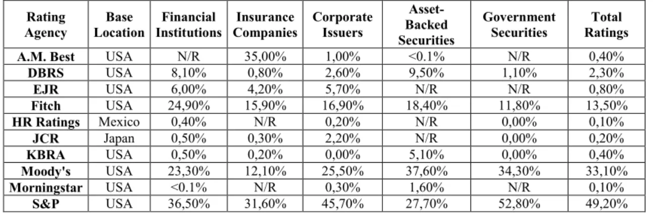
Table 1: Number of Outstanding Credit Ratings as of December 31, 2017 by Rating Category Rating Agency Base Location Financial Institutions Insurance Companies Corporate Issuers Asset-Backed Securities Government Securities Total Ratings A.M. Best USA N/R 7.191 1.079 5 N/R 8.275 DBRS USA 12.730 164 2.938 14.951 18.865 49.648 EJR USA 9.446 864 6.420 N/R N/R 16.730 Fitch USA 39.189 3.261 18.933 29.108 205.674 296.165 HR Ratings Mexico 560 N/R 184 N/R 374 1.118 JCR Japan 839 59 2.464 N/R 440 3.802 KBRA USA 838 32 0 8.110 72 9.052 Moody's USA 36.631 2.484 28.635 59.320 598.614 725.684 Morningstar USA 44 N/R 297 2.530 N/R 2.871 S&P USA 57.091 6.496 51.213 43.760 920.306 1.078.866 Total 157.368 20.551 112.163 157.784 1.744.345 2.192.211

Table 2: Percentage by Rating Category of CRA as of December 31, 2017

Rating Agency Base Location Financial Institutions Insurance Companies Corporate Issuers Asset-Backed Securities Government Securities Total Ratings A.M. Best USA N/R 35,00% 1,00% <0.1% N/R 0,40%

DBRS USA 8,10% 0,80% 2,60% 9,50% 1,10% 2,30% EJR USA 6,00% 4,20% 5,70% N/R N/R 0,80% Fitch USA 24,90% 15,90% 16,90% 18,40% 11,80% 13,50% HR Ratings Mexico 0,40% N/R 0,20% N/R 0,00% 0,10% JCR Japan 0,50% 0,30% 2,20% N/R 0,00% 0,20% KBRA USA 0,50% 0,20% 0,00% 5,10% 0,00% 0,40% Moody's USA 23,30% 12,10% 25,50% 37,60% 34,30% 33,10% Morningstar USA <0.1% N/R 0,30% 1,60% N/R 0,10% S&P USA 36,50% 31,60% 45,70% 27,70% 52,80% 49,20%

2.4. CREDIT RATING PROCESS AND SCALES

Rating agencies report their opinions on several scales. CRs are the most common ones, but CRAs also issue scores and other quantitative opinions about financial and operational performance. CRs for issuers is an insight into an entity's relative capacity to

6

meet financial obligations, such as interest, preferred dividends, principal repayment, insurance claims, or counterpart obligations. CRs provided by rating agencies are forward-looking and only assess the probability of default, that is, the credit risk of an entity.

Investors use CRs as proof of the possibility of earning their money owed in line with the terms and conditions under which they borrowed. Besides, CRs apply to the global scale and securities or other obligations of businesses, the sovereign financial, banks, insurance, and public finance agencies, or structured financing securities backed by claims and other financial assets. (Rating Definitions, 2020)

CRAs present the CRs in relative rank order, but they only reflect the credit risk assessments, which do not forecast a particular rate of default or loss level. While CRAs do not use the same qualitative codes, a correspondence between each organization's rates is usually present as in Table 3. (Afonso, Gomes, & Rother, 2007) In descending order form AAA to CCC, S&P, and Fitch uses identical qualitative keys, while the Moody system runs from Aaa to Caa3. Other than AAA to CCC order scale, other scales exist, for instance, support rating floors from Fitch are using different scales from 1 to 5, but the scales illustrated in Table 3 are the most used rating scale.

CRAs only assess the credit risk; therefore, any risk other than credit risk is addressed directly by CRs. In particular, ratings do not address the risk of a loss of market value in terms of rating security as a result of interest rate changes, liquidity, or operational risk, which may increase the probability of default. (Rating Definitions, 2020)

7

Table 3: Credit Ratings Numerical Scale Correspondence

S&P Moody’s Fitch Scale 21 Scale 17

Highest credit quality

In ve stmen t gr ade

AAA Aaa AAA 21 17

Very high credit quality

AA+ Aa1 AA+ 20 16

AA Aa2 AA 19 15

AA- Aa3 AA- 18 14

High credit quality

A+ A1 A+ 17 13

A A2 A 16 12

A- A3 A- 15 11

Good credit quality

BBB+ Baa1 BBB+ 14 10 BBB Baa2 BBB 13 9 BBB- Baa3 BBB- 12 8 Speculative Spec ula tive g ra de BB+ Ba2 BB+ 11 7 BB Ba2 BB 10 6 BB- Ba3 BB- 9 5 Highly speculative B+ B1 B+ 8 B B2 B 7 B- B3 B- 6

Substantial credit risk.

CCC+ Caa1 CCC+ 5

CCC Caa2 CCC 4

CCC- Caa3 CCC- 3

Very high levels of credit risk CC Ca CC

2 C Default SD C DDD D DD 1 D

2.5. SYSTEMIC RISK

One of the most commonly used terms is the systemic risk due to the global economic crisis in the world economy, especially after the 2008 global financial crisis. Systemic risk is one reason why the crisis started at one point and quickly spread to the global economy as happened in the 2008 global financial crisis. The crisis started in the United States of America due to mortgage loans, but then it became a global financial crisis.

Systemic risk refers to the risk that the failure of a single entity or cluster of entities can lead to a failure that could potentially bankrupt or disrupt the entire system due to interconnections and interdependence. Systemic risk can be described as the possibility or likelihood of a complete system failure. When a systemic risk occurs, it will affect every part of the economy, eventually like domino stones. Therefore, the systemic danger

8

of bank failures in a single country can spread to several countries or across the globe due to strong correlation and clustering. (Kaufman & Scott, 2003)

According to the report named “Guidance to Assess the Systemic Importance of Financial Institutions” submitted by International Monetary Fund (IMF), Bank for International Settlements (BIS) and Financial Stability Board (FSB) to G20 Finance Ministers and Governors in 2009, systemic risk is defined as follow; a risk of disruption to financial services that is caused by an impairment of all or parts of the financial system and has the potential to have serious negative consequences for the real economy. (FSB, IMF, & BIS, 2009)

Systemic risk has been associated with the banks, which has a gradual impact on other banks due to the first troubled bank default to pay its obligations causes a gradual failure. When the first bank fails to pay its debts to other banks, it created stress on other banks since if they cannot collect their debts, they cannot pay their debts to other banks, continuing until the whole banking system goes bankrupt. Also, when depositors perceived the effects of default fluctuations, liquidity concerns increased throughout banks, a panic may spread among depositors, and many customers may want their money out of a bank because they think that the bank will stop their operations in the near future. The attitude of customers is also called a bank run or run on the bank; many clients withdraw cash from their financial institution's savings accounts at once. Bank run will worsen the banks' status and push banks to sell their liquid and illiquid assets, which may cause a decrease in the value of financial assets, and in return, it triggers another gradual impact on banks since many banks have financial assets in their balance sheet. However, in such circumstances, there will be more sellers than buyers, which gives rise to a sharp decrease in bond prices, stock markets, and other financial assets. As a last resort, the banks have to recall loans extended to the real economy to save themselves, and this, in return, triggers the collapse of the real economy and causes defaults of companies. Because of these interconnections between banks and other banks and customers with banks, policymakers should take account of systemic risk while making policies to protect the financial system.

9

2.6. TOO BIG TO FAIL AND SYSTEMICALLY IMPORTANT

FINANCIAL INSTITUTIONS

Although it is not a new concept, with the global crisis that started in 2008, the TBTF problem was put on the public policymaker's agenda. The TBTF theory says that some firms, particularly financial institutions, are so massive and interconnected that their failure will provoke the collapse of the economic system; therefore, when faced with possible failures, they have to be saved by the government. (Lin, 2010) TBTF type organizations refer to organizations whose bankruptcy is not allowed by governments due to their size and wide-ranging economic and organic relationships with the financial and real economy. In case of bankruptcy, the externalities stemmed from them will reveal financial markets and the real economy and trigger a systemic collapse, as stated in the previous chapter.

As the financial crisis of 2007–2008 unfolded, the international community moved to protect the global financial system through preventing the failure of TBFT, or, if one does fail, limiting the adverse effects of its failure. The United States of America started a program named Troubled Asset Relief Program (TARP), which aims to promote financial market stability during the 2008 global financial crisis. The TARP program originally was projected as a $700 billion budget and authorized the United States government to purchase troubled assets and equity from financial institutions to prevent systemic risk and complete financial failure. Other countries affected by the 2008 global financial crisis also took similar measures to stabilize the financial markets. These programs helped the financial markets to stabilize; however, every action has a price. Despite the fact that governments' actions helped to ease the financial crisis in the short run, the costs of these actions exceeded its benefits in the long run. (Strahan, 2013) These actions could encourage TBFTs to take more risk for making more profit since they know that if everything goes wrong, governments have to save them. Knowing that the government will save TBTFs at all costs increase the risk appetite of them. Likewise, from the investor side, it also encourages investors to provide financing without paying enough attention to the risk profile of the TBTF since they believe the government will shield them from the failure; for these reasons, TBTFs are benefiting from the implicit guarantees from the government. Since they are perceived as guaranteed by governments, they enjoy a competitive advantage over smaller institutions. (Dam & Koetter, 2012) This

10

situation, like the vicious circle, increases implicit guarantees as institutions grow, institutions take more risks as implicit guarantees increase, and systematic risk increases as they take more risk and grow more.

Although TBFT is a serious concern for governments and authorities in times of crisis, it is not easy to define them as there are no clear TBTF criteria, the most obvious criteria are the institutions' size, but it is not sufficient to classify big institutions as TBTF. The interconnectedness of any institutions will also matter for being counted as TBFT. TBTF is a broader term that includes banks, insurance companies, financial institutions, and other institutions that might cause systemic risk.

TBTF is always associated with SIFIs, and SIFI refers to the financial institutions whose failure might trigger a financial crisis as TBTFs. Currently, a standard definition of SIFI had not been decided yet. However, the Basel Committee, which is a committee of banking supervisory authorities that was established by the central bank governors of 45 members from 28 Jurisdictions, consisting of Central Banks and authorities with responsibility of banking regulation, has identified factors for assessing whether a financial institution is systemically important. These factors are size, complexity, interconnectedness, the lack of readily available substitutes for the financial infrastructure it provides, and its global activity. (Bank for International Settlements, 2020)

In this study, the support rating published by The Fitch rating agency has been used as a proxy variable for SIFIs, since there is no agreed objective method of measurement of the institution's systemic importance. It is accepted that if an institution's support rating is high, it indicates that that institution has higher systemic importance.

11

3. LITERATURE REVIEW

After the 2008 global financial crisis, the implicit guarantees from governments to SIFI gained public interest since it creates a conflict of interest between taxpayers and SIFIs. Scholars around the world tried to quantify this implicit guarantee, and some of them proposed additional tax or levy for SIFIs to cover the damage they might cause in times of crisis.

Doluca, Ulrich, and Maruo (2010) tried to find the optimum tax rate, which would efficiently and globally reduce the systemic risk. According to them, systemic importance should be compensated with a tax, and the level of tax should be rose with the systemic importance of an institution. Besides, they proposed establishing a systemic risk fund to use this fund for rescuing SIFI in case of any crisis stemming from systemic risks. This fund should be established through the compensation tax proceed mentioned above. In this way, it might prevent moral hazard issues and conflict of interest between taxpayers and SIFIs. However, it is hard to quantify this type of tax; there will be thresholds for institutions, and if these thresholds are not balanced well, it will hinder economies of scale and might do more harm than its benefits. Also, it should be implemented on a global scale; otherwise, the global competitiveness of banks operating in a country where this tax is applied may decrease.

Baker and McArthur (2009) asserted that the implicit subsidies that provide funding cost advantage ranges from 9 to 49 bp to SIFI compared to small institutions or systemically not important institutions. They analyzed the price difference in funding costs between small and large U.S. banks before and after TARP. However, this method's price differences cannot be entirely explained because TARP was an extreme interference to the market and destroyed all the market dynamics. Therefore, it is not enough to explain the funding cost advantages of implicit subsidies in tranquil times.

Acharya, Anginer, and Warburton (2016) analyzed TBTFs between 1990-2012 such a long period, including the 2008 global financial crisis. They both used bonds spreads traded in the U.S. between 1990 and 2012 and ratings of larger and smaller companies assigned CRAs. They also compared big financial companies with non-financial firms to control the effects of size on bond spreads. They find that government

12

guarantees are embedded in the credit spreads of bonds issued by large U.S. financial institutions, while larger non-financial institutions do not enjoy implicit government guarantees. The relationship between firm size and bond spreads is not seen in non-financial sectors, as seen in non-financial sectors.

Ueda and Mauro (2013) used CRs to identify the implicit government guarantees to SIFIs and tried to estimate the value of the subsidy, embedded in CRs of institutions in their study. Since they found an important implicit government subsidy in CRs which provide funding cost advantages, as Doluca, Ulrich, and Maruo (2010) did, they also proposed a SIFI tax for compensating that advantage that would help decreased their tendency to become broad and complex.

Other than credit spreads and CRs approach to defining implicit government guarantees, Ghandi and Lustig (2015) examined equity data of SIFIs to find out the effects of implicit subsidy to stocks of SIFIs. According to their study, even if there are implicit government guarantees to SIFIs, it is not perceived by shareholders.

There are many studies for determining the implicit government guarantees to SIFIs; some of them used bonds or credit spreads, some used equity, and some used CRs. In my study, I chose to use ratings since I think that CRs have some advantages over bond spreads or equity prices. The most obvious advantage is that spread or equity prices can be easily affected by market conditions. Liquidity crisis or political crisis or news can affect both spreads and equity prices in a short time; however, CRs assigned after detailed quantitative and qualitative analysis. Therefore, CRs cannot be affected by market conditions as quickly affected as bond spreads or equity prices.

13

4. DATA DESCRIPTION

4.1. REFERENCE CREDIT RATINGS

In order to quantify implicit government guarantees to the SIFIs, I benefited from Fitch Ratings. The reason for using Fitch ratings is that they provide several kinds of ratings assessing the financial stability or creditableness of any institutions from various aspects that will allow me to distinguish the effect of government support. In this study, used CRs are as follows: Sovereign Long-Term Rating, Issuer Long-Term Rating, Support Rating, Support Rating Floor, and Viability Rating.

4.1.1. Sovereign Long-Term Rating

A Sovereign Long-Term Rating (SLTR) provides an objective evaluation of a country's creditworthiness and may provide investors with insights into the level of risk associated with a country that reflects the overall vulnerability to default. SLTR also takes into account political risks. (Kronwald, 2009) SLTRs are generally crucial for those countries who want to be available on international bond markets or draw foreign direct investment. These grades are given from AAA (highest) to D (lowest), and I used the 21 numerical rating scale, which is stated in Table 3 for this study. 21 is representing AAA, and 1 is representing D.

4.1.2. Issuer Long-Term Ratings

Issuer Long Term Rating (ILTR) is similar to SLTRs; their scales and definitions are the same except for that these are assigned to entities. Entities usually cannot be rated higher than the countries in which they operate, even though the entities have better more creditworthiness. (Rating Definitions, 2020) The reason for that rule is that any entity's financial performance is mainly dependent on the country’s performance. There is a strong correlation between a country’s performance and entity performance. Issuer ILTRs also be graded from AAA to D, and for this study, 21 numerical scales are used.

14

4.1.3. Support Rating

Support Ratings (SRs) reflect the Fitch's view on the probability that a financial institution will receive support to prevent it from defaulting on its senior obligations in case of needs. This support might come from one of two sources: shareholders of the entity or national authorities of the country in which the entity operates. In some cases, SRs may also represent potential support from other sources, such as foreign financial institutions. SR is scaled to 1 to 5. As explained before in previous, SR is accepted as a proxy variable to measure the systemic importance of an institution.

1: An extremely high probability of external support. The potential provider of support is very highly rated in its own right and has a very high propensity to support the bank in question. This probability of support indicates a minimum Long-Term Rating floor of ‘A–’.

2: A high probability of external support. The potential provider of support is highly rated in its own right and has a high propensity to provide support to the bank in question. This probability of support indicates a Long-Term Rating floor in the ‘BBB’ category

3: A moderate probability of support because of uncertainties about the ability or propensity of the potential provider of support to do so. This probability of support indicates a Long-Term Rating floor in the ‘BB’ category.

4: A limited probability of support because of significant uncertainties about the ability or propensity of any possible provider of support to do so. This probability of support indicates a Long-Term Rating floor of ‘B+’ or ‘B’.

5: A possibility of external support, but it cannot be relied upon. This may be due to a lack of propensity to provide support or to very weak financial ability to do so. This probability of support indicates a Long-Term Rating floor no higher than ‘B–’ and in many cases, no floor at all. (Rating Definitions, 2020)

15

4.1.4. Support Rating Floor

The Support Rating Floors (SRFs) represents Fitch’s view on the probability of extraordinary support, particularly from government authorities, in case of need. While assigning SFR generally national authorities of the country where the financial institution operates is taken into account, but sometimes Fitch may take into account international government institutions into its assessment. Thus, SRFs do not capture the institutional support potential from shareholders of the entity. (Rating Definitions, 2020) SLTR credit ranking system applies to SRFs, which is scaled AAA to D. Where there is no solid expectation that there would be sovereign assistance, it is given a 'No Floor'.

4.1.5. Viability Rating

Viability ratings (VRs) measure a financial institution's intrinsic creditworthiness and reflect Fitch's opinion on the probability of the entity failing. While assigning VRs, Fitch distinguishes between "ordinary support", which a bank benefits thanks to the ordinary course of operation, and "extraordinary support" given to a failed bank to pay its obligations. Ordinary support is taken into account in a bank's VR, while extraordinary support is related to SR and/or SRF and captured in these ratings. Ordinary support means that the benefits accrued to all banks as a result of their position as banks, including regular access to liquidity from central banks in line with those on the market. Similar to ILTRs, VRs reflect risks arising from the countries in which the entity operates as well.

VRs are assigned on a scale that is the same as the AAA to D, but there is no D rating on the VR scale; instead of it, there is an F rating at the lower, and it shows Fitch's opinion that a bank has failed. (Rating Definitions, 2020)

16

4.2. COLLECTED DATA

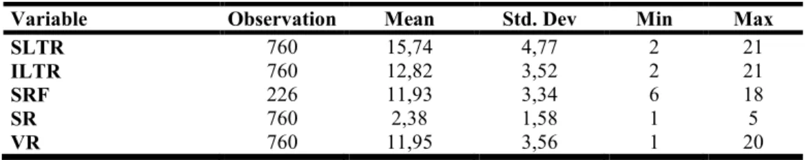
For this study, I collected 3266 CR published by Fitch Ratings at the year-end of 2019 for 760 distinct banks from 90 countries. These data are publicly available on the official website of Fitch Ratings. Twenty-five of these countries are classified as developed countries, and the rest are developing countries, according to the World Bank’s country classification. Tables 4 and 5 show the distribution of the sample by country and summary statistics of the data collected. In this study, CRs are used in their 21-scale numerical form, which is shown in Table 3 except for SR. For SR, which is scaled 1-5 (1 is highest, and 5 is lowest), I used flipped values. The highest probability of support is denoted as 5, and the lowest is 1 in order to achieve healthy results in regression analysis.

Table 6 shows the comparison of developed and developing countries in terms of SR and SFR. In developed countries, SRF is higher than in developing countries, and it is due to developed countries have higher STLR, which allows them to have higher SRF. However, regarding SR, the banks operated in developing countries are enjoying higher SRs. Since SR comes from either shareholders or national authorities, although SRF is low in developing countries, higher SR means this support comes from shareholders. It can be partly explained by the fact that some of the banks operating in developing countries are either owned by larger banks in developed countries or have a share in the equity of larger banks. Another explanation for higher SR could be that banks in developing countries are controlled by those who are capable of putting pressure on governments to support the banks in times of a crisis.

17 Table 4: Distribution of the Sample by Country

Countries Sample Percent Countries Sample Percent

Andorra 3 0,39% _Kenya 3 0,39% Argentina 6 0,79% _Korea* 8 1,05% Armenia 2 0,26% _Kuwait 11 1,45% Australia* 14 1,84% _Lebanon 2 0,26% Austria* 4 0,53% _Luxembourg* 3 0,39% Azerbaijan 3 0,39% _Macao 1 0,13% Bahrain 5 0,66% _Malaysia 2 0,26% Belarus 5 0,66% _Malta 2 0,26% Belgium* 5 0,66% _Mexico 13 1,71% Bolivia 2 0,26% _Mongolia 2 0,26% Brazil 16 2,11% _Morocco 3 0,39% Bulgaria 6 0,79% _Netherlands* 10 1,32%

Cameroon 1 0,13% _{New Zealand*} 14 1,84%

Canada* 9 1,18% _Nigeria 10 1,32%

Chile 6 0,79% _Macedonia 1 0,13%

China 16 2,11% _Norway* 4 0,53%

Colombia 9 1,18% _Oman 6 0,79%

Costa Rica 4 0,53% _Panama 11 1,45%

Croatia 1 0,13% _Peru 5 0,66%

Cyprus 2 0,26% _Philippines 8 1,05%

Czech Republic 2 0,26% _Poland 9 1,18%

Denmark* 3 0,39% _Portugal* 6 0,79%

Dominican Republic 2 0,26% _Qatar 8 1,05%

Ecuador 3 0,39% _Romania 5 0,66%

Egypt 2 0,26% _Russia 29 3,82%

El Salvador 2 0,26% _{Saudi Arabia} 10 1,32%

Finland* 1 0,13% _Serbia 1 0,13%

France* 14 1,84% _Singapore* 5 0,66%

Georgia 7 0,92% _Slovenia 4 0,53%

Germany* 16 2,11% _{South Africa} 9 1,18%

Ghana 1 0,13% _Spain* 20 2,63%

Greece 4 0,53% _{Sri Lanka} 2 0,26%

Guatemala 5 0,66% _Sweden* 5 0,66%

Hong Kong* 10 1,32% _Switzerland* 12 1,58%

Hungary 3 0,39% _Taiwan 18 2,37%

India 8 1,05% _Thailand 8 1,05%

Indonesia 10 1,32% _Tunisia 1 0,13%

Iraq 1 0,13% _Turkey 25 3,29%

Ireland* 5 0,66% _Ukraine 9 1,18%

Israel* 2 0,26% _{United Arab Emirates} 17 2,24%

Italy* 14 1,84% _{The United Kingdom*} 35 4,61%

Jamaica 1 0,13% _{United States*} 129 16,97%

Japan* 14 1,84% _Uruguay 3 0,39%

Jordan 3 0,39% _Uzbekistan 8 1,05%

Kazakhstan 7 0,92% _Vietnam 4 0,53%

Total 259 34,08% Total 760 100%

18 Table 5: Summary Statistics for Credit Ratings.

Variable Observation Mean Std. Dev Min Max

SLTR 760 15,74 4,77 2 21

ILTR 760 12,82 3,52 2 21

SRF 226 11,93 3,34 6 18

SR 760 2,38 1,58 1 5

VR 760 11,95 3,56 1 20

Table 6: Summary Statistic by Country Groups

Observation Mean Std. Dev

SRF SR SRF SR SRF SR

Developing Countries 189 398 11,42 2,76 3,30 1,42

Developed Countries 37 362 14,54 1,96 2,14 1,65

Total 226 760 11,93 2,38 3,34 1,58

5. DESCRIPTIVE STATISTICS

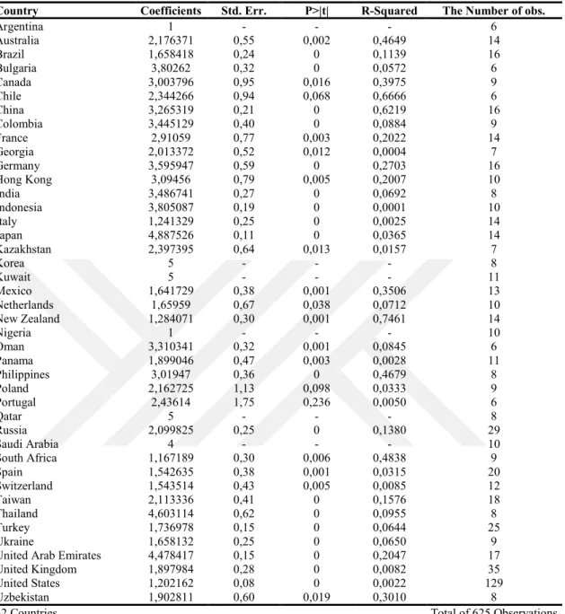
It is thought by most people that the support provided to SIFIs by governments is directly proportional to the size, and I also thought it might be. Simple ordinary least squares regression was conducted to show the relationship between size and level of support for each country whose sample includes more than six banks. Limiting samples with countries with more than 6 samples is required for getting a healthy result from regression, and it is a criterion set by me. The regression analysis was conducted for 42 countries out of 90. Banks’ assets size to GDP ratio was used as the independent variable, and SR was used as the dependent variable. While banks’ asset size obtained from the Fitch website, the GDP of countries obtained from the World Bank website. However, Table 7 proves that there is no statistically significant relationship between size and level of support for most countries, and asset size is not the primary determinant for counting as SIFI.

19

Table 7: Results of SR and Banks Asset Size Relationship

Country Coefficients Std. Err. P>|t| R-Squared The Number of obs.

Argentina 1 - - - 6 Australia 2,176371 0,55 0,002 0,4649 14 Brazil 1,658418 0,24 0 0,1139 16 Bulgaria 3,80262 0,32 0 0,0572 6 Canada 3,003796 0,95 0,016 0,3975 9 Chile 2,344266 0,94 0,068 0,6666 6 China 3,265319 0,21 0 0,6219 16 Colombia 3,445129 0,40 0 0,0884 9 France 2,91059 0,77 0,003 0,2022 14 Georgia 2,013372 0,52 0,012 0,0004 7 Germany 3,595947 0,59 0 0,2703 16 Hong Kong 3,09456 0,79 0,005 0,2007 10 India 3,486741 0,27 0 0,0692 8 Indonesia 3,805087 0,19 0 0,0001 10 Italy 1,241329 0,25 0 0,0025 14 Japan 4,887526 0,11 0 0,0365 14 Kazakhstan 2,397395 0,64 0,013 0,0157 7 Korea 5 - - - 8 Kuwait 5 - - - 11 Mexico 1,641729 0,38 0,001 0,3506 13 Netherlands 1,65959 0,67 0,038 0,0712 10 New Zealand 1,284071 0,30 0,001 0,7461 14 Nigeria 1 - - - 10 Oman 3,310341 0,32 0,001 0,0845 6 Panama 1,899046 0,47 0,003 0,0028 11 Philippines 3,01947 0,36 0 0,4679 8 Poland 2,162725 1,13 0,098 0,0333 9 Portugal 2,43614 1,75 0,236 0,0050 6 Qatar 5 - - - 8 Russia 2,099825 0,25 0 0,1380 29 Saudi Arabia 4 - - - 10 South Africa 1,167189 0,30 0,006 0,4838 9 Spain 1,542635 0,38 0,001 0,0315 20 Switzerland 1,543514 0,43 0,005 0,0085 12 Taiwan 2,113336 0,41 0 0,1576 18 Thailand 4,603114 0,62 0 0,0955 8 Turkey 1,736978 0,15 0 0,0644 25 Ukraine 1,658132 0,25 0 0,0650 9 United Arab Emirates 4,478417 0,15 0 0,2047 17 United Kingdom 1,897984 0,28 0 0,0082 35 United States 1,202162 0,08 0 0,0022 129 Uzbekistan 1,902811 0,60 0,019 0,3010 8

20

5.1. REGRESSION ANALYSIS

ILTR of a bank can be explained by two variables: the first one is VR, which reflects the intrinsic value of a bank, and the other one is SR, which reflects the expected support in case of need. To quantify the effects of these two variables to ILTR, I conducted an Ordered Probit Model (OP). Since dependent variables are in categorical form, OP is the most suitable model for my data. The OP explains the variation of the ordered categorical dependent variable as a function of one or more independent variables. It is used to classify the different categories (e.g., the lowest to highest, strongly agree to strongly disagree). The other possible method which can be used for my data is Ordinary Least Square (OLS) model. However, since I have 21 categories (from scale 1 to 21), OLS will assume that the distance between the 21 categories is all equal, which can be a problem for the result, but OP model relaxes that assumption. My regression can be formulated as equation 1. My dependent variable is ILTR, which is the overall rating of the banks. The dependent variables are SR and VR, which denote respectively expected support and intrinsic rating or stand-alone rating of a bank. I also added SLTR because it is the other factor determining the ILTR due to the country ceiling. CRAs using SLTR notes as country ceilings, which defines the maximum CR achievable for an entity in a particular country. As explained before, the country ceiling is that an entity operates in a particular country has the same risk exposure that country has; therefore, STLR is one of the main determinants of the ILTR. Since there is a debate between statisticians regarding the fixed effect in OP, I run regression twice with and without a fixed country effect. OP models are stated as a probability equation, as stated in equation 1. In the equation, F denoting normal cumulative density function, “i” denotes banks in a particular “k” country. The equation below structured for country fixed effect regression, for regular regression “α3SLTRk” defined as “α3SLTRki”. I have 20 ILTR ratings for 760 banks starting from C (2) to AAA (21) so that there are 19 thresholds to from lowest rating to highest, which are called cut points and for the smallest rating equation should be as equation 2 and for the highest rating as equation 3.

Equation 1: Prob (ILTRik = x) = F (α1 SRik + α2 VRik + α3SLTRk ≤ cutx) –

F (α1 SRik + α2 VRik + α3SLTRk ≤ cutx-1)

21

Equation 3: Prob (ILTRik = 20) = 1- F (α1 SRik + α2 VRik + α3SLTRk ≤ cut19)

As can be seen from Table 8, the results of the model with country fixed effect have better pseudo R-sq, while the results of the model without country fixed effects provide better P values for variables and breakpoints; therefore, I think it would be more useful to interpret both results together.

The results of the regressions are similar to each other, as can be seen from columns 1 and 5 of Table 8. Column 1 is indicating the results of the regression with country fixed effect, and column 5 is for without the country fixed-effect model. The coefficient of SR (α1) is 0,622 in column 1, and 0,606 in column 5. Each regression indicates that an increase in support rate will also increase ILTR.

Since I have 20 categorical results and 19 cut-points, there are 18 steps from the lowest rating to the highest rating. Therefore, for simplification, we can divide the difference between the highest cut-point and the lowest cut-point into the number of steps to find the average score required to cross a cut-point. Average cut-points (=(Cut19-Cut1)/18) are 29,5/18=1,63, and 17,2/18=0,95 for column 1 and column 5, respectively, these figures indicate the average score required to have one notch higher rating. Although cut points distances are not equal as stated before, I used average cut-point difference for simplification, for example, between cut18 and cut19 of column 1 there are only 0,42 points while cut5 and cut6 of column 1 there are 1,831 points and it means that government support is more valuable at higher ratings.

When all other variables (VR and STLR) are constant, assuming only SR changes, a notch increase in SR will reflect the increase in ILTR around 0,38 (0,622/1,63) notches according to α1 (coefficient of SR) from column 1. According to α1 (coefficient of SR) from column 5, the increase is about 0,63 (0,606/0,95) notches. It should be known that these figures indicate approximate increases because the differences between cut points are not equal.

22 Table 8: Results of Ordered Probit Regression

Country Fixed Effects No Fixed Effects

1 2 3 4 5 6 7 8 VR 1,005*** 1,003*** 1,022*** 1,024*** 0,614*** 0,691*** 0,655*** 0,715*** (6,41) (6,26) (6,64) (6,64) (12,33) (9,72) (12,62) (9,88) SR 0,622*** 0,526*** 0,755*** 0,719*** 0,606*** 0,396*** 0,758*** 0,505*** (12,10) (8,90) (10,40) (7,25) (20,13) (10,96) (16,74) (6,94) SLTR 0,361*** 0,361*** 0,296*** 0,333*** 0,213*** 0,226*** 0,202*** 0,212*** (6,35) (6,68) (4,35) (5,34) (12,04) (12,26) (11,45) (10,93) Dev 3,104** 2,940** -1,227*** -1,258*** (3,21) (3,00) (-5,51) (-5,43) Dev*SR 0,332** 0,215 0,598*** 0,589*** (3,17) (1,36) (7,01) (4,71) Parent 0,446** 0,420** 0,476*** 0,288* (3,23) (2,99) (3,58) (2,13) Parent*SR -0,218** -0,154 -0,285*** -0,206** (-2,93) (-1,93) (-4,69) (-3,11) Parent*SR*Dev -0,130 0,0276 (-1,28) (0,32) cut1 -3,735** 0,236 -4,397** -0,184 2,030*** 1,499** 2,308*** 1,608*** (-2,68) (0,12) (-3,02) (-0,09) (5,26) (3,25) (5,78) (3,52) cut2 -2,765* 1,205 -3,442* 0,767 2,746*** 2,276*** 3,021*** 2,380*** (-1,99) (0,59) (-2,36) (0,37) (6,76) (4,49) (7,29) (4,81) cut3 3,358* 7,213*** 2,737* 6,847** 4,120*** 3,835*** 4,426*** 3,931*** (2,57) (3,47) (1,98) (3,27) (14,88) (8,71) (15,10) (9,27) cut4 4,845*** 8,618*** 4,240** 8,270*** 4,594*** 4,365*** 4,921*** 4,467*** (3,94) (4,09) (3,20) (3,94) (14,69) (8,99) (14,84) (9,50) cut5 7,664*** 11,41*** 7,113*** 11,12*** 5,805*** 5,744*** 6,186*** 5,870*** (5,43) (4,90) (4,69) (4,84) (18,75) (11,27) (18,54) (11,95) cut6 9,495*** 13,29*** 8,968*** 13,03*** 7,011*** 7,129*** 7,443*** 7,279*** (6,30) (5,44) (5,57) (5,44) (21,08) (12,53) (20,62) (13,28) cut7 11,25*** 15,12*** 10,76*** 14,90*** 8,230*** 8,556*** 8,711*** 8,730*** (7,04) (5,94) (6,35) (6,00) (22,18) (13,47) (21,57) (14,21) cut8 12,63*** 16,54*** 12,15*** 16,34*** 9,215*** 9,725*** 9,725*** 9,909*** (7,46) (6,24) (6,79) (6,34) (22,36) (13,90) (21,74) (14,60) cut9 13,65*** 17,60*** 13,18*** 17,40*** 9,950*** 10,60*** 10,47*** 10,78*** (7,64) (6,40) (7,00) (6,52) (22,14) (14,00) (21,62) (14,67) cut10 14,89*** 18,89*** 14,42*** 18,70*** 10,85*** 11,68*** 11,39*** 11,86*** (7,89) (6,61) (7,27) (6,74) (22,40) (14,35) (21,91) (15,04) cut11 16,13*** 20,18*** 15,67*** 20,00*** 11,81*** 12,79*** 12,36*** 12,99*** (8,03) (6,76) (7,45) (6,91) (22,46) (14,55) (21,98) (15,18) cut12 17,38*** 21,45*** 16,92*** 21,28*** 12,80*** 13,86*** 13,37*** 14,06*** (8,18) (6,91) (7,63) (7,08) (22,49) (14,80) (22,02) (15,40) cut13 18,68*** 22,76*** 18,23*** 22,60*** 13,87*** 14,97*** 14,48*** 15,20*** (8,26) (7,01) (7,74) (7,21) (22,42) (14,89) (21,95) (15,47) cut14 19,90*** 23,99*** 19,46*** 23,85*** 14,70*** 15,84*** 15,34*** 16,09*** (8,46) (7,19) (7,98) (7,41) (23,08) (15,49) (22,66) (16,07) cut15 21,09*** 25,16*** 20,66*** 25,02*** 15,48*** 16,67*** 16,13*** 16,92*** (8,59) (7,31) (8,12) (7,54) (23,76) (15,96) (23,18) (16,48) cut16 22,31*** 26,35*** 21,89*** 26,23*** 16,40*** 17,58*** 17,07*** 17,85*** (8,71) (7,44) (8,28) (7,69) (24,29) (16,26) (23,73) (16,81) cut17 23,91*** 27,94*** 23,58*** 27,92*** 17,79*** 18,96*** 18,56*** 19,30*** (8,80) (7,56) (8,42) (7,85) (23,75) (16,34) (23,31) (16,98) cut18 25,29*** 29,28*** 25,00*** 29,33*** 18,82*** 20,02*** 19,64*** 20,38*** (9,00) (7,75) (8,66) (8,09) (23,06) (16,39) (22,92) (17,07) cut19 25,72*** 29,69*** 25,49*** 29,82*** 19,19*** 20,34*** 20,06*** 20,73*** (9,06) (7,81) (8,76) (8,21) (23,26) (16,40) (23,00) (17,22) N 760 760 760 760 760 760 760 760 pseudo R-sq 0,545 0,549 0,548 0,553 0,433 0,464 0,443 0,469 t statistics in parentheses * _{p < 0,05,} ** _{p < 0,01,} *** _{p < 0,001}

23

To explain the result of the regression better and have a more comfortable understanding, I used the 2019 year-end ratings of Industrial and Commercial Bank of China Limited (ICBC) in the current formula (“α1 SRik + α2 VRik + α3SLTRk”). ICBC's 2019 year-end ILTR is “A”, which corresponds numerically to 16. According to the result of OP model shown in the first column of Table 8, in order to have “A” ILTR (category 16), a bank should have combined score from the above equation between the values of cut14 and cut15 (crossing cut1 means category 3 and crossing cut19 means category 21 since the ratings starting from C (2) to AAA (21) ). This combined score should be between 19,90 and 21,09. As seen in Table 9, column 1 represents the credit ratings of ICBC; column 2 represents the coefficients of relevant credit ratings. Moreover, the third column refers to the values that result from multiplying the first and the second column and the total combined score of the ICBC. ICBC’s combined score is 20,302, which is exceeding the value of cut14 but below cut15. Therefore according to the result of the regression, ICBC’s rating corresponds to category 16 (ILTR=A in alphabetical scale), which is also actual rating at the year-end of 2019. If ICBC’s combined score exceeds 21,09 (cut15), it should have a rating of category 17, which corresponds “A+”.

Table 9: Credit Ratings of ICBC

Industrial and Commercial Bank of China Limited Regression Results

1 2 3

21 Numerical Scale Correspondence Coefficients Impact on Equation

VR 11 1,005 11,055

SR 5 0,622 3,11

SLTR 17 0,361 6,137

24

5.2. ROBUSTNESS CHECKS VIA DUMMY VARIABLES

Support levels of developing and developed countries to their banks may differ because developed and developing countries have different market dynamics. For example, banks in developing countries may be owned by people close to the government or large families that can pressure the government, which can affect the degree of support. Therefore, a dummy variable was created to measure the effects of support from developing countries and developed countries separately. Developing countries have been marked with “1” in the regression, and a variable created named “Devik.” o isolate developed country support effect, another variable created and denoted as “Devik* SRik”. The equation is structured again as and Equation 4.

Equation 4: Prob (ILTRik = x) = F (α1 SRik + α2 VRik +α3SLTRk +α4 Devik +α5 Devik* SRik

≤ cutx) –

F (α1 SRik + α2 VRik +α3SLTRk +α4 Devik +α5 Devik* SRik ≤ cutx-1)

Regression was conducted twice with and without fixed effects, and now coefficient “α5” indicates the additional effects of developing countries' support, while “α1” indicates the solely developed countries' support. As seen in columns 2 and 6 of Table 8, there is additional positive support from developing countries; the coefficient “α5” indicates this additional support, which is 0,332 and 0,598, respectively. When all other variables (VR and STLR) are constant, assuming only SR changes, one notch increase in SR will reflect around 0,32 (0,526/1,63) notches the increase in the ILTR in developed countries, according to “α1” (coefficient of SR) in column 2, and around 0,38 (0,396/1,04) notches increase according to “α1” from column 6. For developing countries, there is additional effect which are 0,20 (0,332/1,63) for fixed effect and 0,57 (0,598/1,04) notches for regular regression. According to the results of both regressions, SR is more valuable in developing countries. Although there is little deviation between the results of equation 1 and equation 4, they are still consistent in direction, and this deviation may be a result of the simplification.

25

In some cases, SR includes parent company support, and to exclude parent support from SR, another dummy variable was created and denoted as "Parent", and the entities with parent company marked with “1". The regression equation is structured as equation 5. Now coefficient “α1” only reflects pure government support, whether it comes from developed or developing countries and “Parentik* SRik” variable created to isolate parent company effect and coefficient of this variable, “α7”, is reflecting additional parent support effect. Again, the regression was conducted twice with/without country fixed effect.

Equation 5: Prob (ILTRik = x) = F (α1 SRik + α2 VRik +α3SLTRk +α6 Parentik +α7

Parentik* SRik ≤ cutx) –

F (α1 SRik + α2 VRik +α3SLTRk +α6 Parentik +α7 Parentik* SRik ≤ cutx-1)

As seen from columns 3 and 7 of Table 8 and surprisingly, additional parent company coefficient “α7” is negative in both results. Coefficient “α7” is -0.218 and -0.285 in columns 3 and 7, respectively, and it means that having a parent company will result in to decrease in ILTR. According to the result of equation 5, Coefficient “α1” is 0,755 and 0,758, respectively, in columns 3 and 7. There is a slight increase in coefficient, and it is due to the negative parent company coefficient. However, still, the direction and the value of SR coefficient have not deviated so much. When all other variables are constant, only the SR changes, one notch increase in SR will reflect around 0,45 (0,75/1,66) notches the increase in the ILTR in developed countries, according to “α1” from column 3, and around 0,76 (0,758/0,98) notches increase according to “α1” from column 7.

To separate the support of developed countries, developing countries, and parent company, I combined developing and parent dummy and established a new variable denoted as “Devik*Parentik*SRik” and the equation is structured as Equation 6. Now, the “α1” coefficient now only captures the pure government support effect of developed countries. Coefficient “α5” and “α7” stand for additional developing country effects and additional parent company effects. The new coefficient “α8” is a combination of developing and parent company effect.

Equation 6: Prob (ILTRik = x) = F (α1 SRik + α2 VRik +α3SLTRk + α4 Devik +α5 Devik*SRik

26

F (α1 SRik + α2 VRik +α3SLTRk + α4 Devik +α5 Devik*SRik +α6 Parentik +α7

Parentik*SRik + α8Devik*Parentik*SRik ≤ cutx-1)

The regression was conducted twice, with/without country fixed effect. As seen in columns 4 and 8 from Table 8, the results are still consistent with little deviation. Again, when all other variables are constant, only if the SR changes, one notch increase in SR will reflect around 0,43 (0,72/1,66) notches the increase in the ILTR in developed countries, according to “α1” from column 4, and around 0,47 (0,51/1,06) notches increase according to “α1” from column 8.

5.3. ROBUSTNESS CHECKS VIA SUBGROUPS

Although using dummy variables for measuring the effects of every subgroup in one regression equation is a robust way, it may be more accurate to create separate models if the characteristics of all subgroups are very different from each other. Therefore, I created 5 different groups by dropping samples. The first group is only for developing countries; I dropped samples from developed countries and achieved 398 samples. For the second group, I deleted the banks' data who have a parent company from the first group, and the banks operating in developing countries without a parent company remained in my sample. For the third group, the samples from developing countries are removed, and 362 samples are left. For the fourth group, as did for the second group, samples with parent companies are deleted, and the data of the banks operating in developed countries without parent company remained in my sample. For the last group, the banks' data with parent company are deleted, and the banks operate in developing or developed countries without a parent company remaining in my sample.

To sum up, the groups can be described respectively as the banks from developing countries, the banks from developing countries without a parent company, the banks from developed countries, the banks from developed countries without a parent company, and the banks without a parent company. SR data in the last group reflect pure government support because, in the absence of a parent company, the support only comes from the government. I used a similar approach for the regression analysis; two different regression models with equation 1 are used, which are with and without country fixed effect OP model. I conducted 10 separate regression analyses for five groups, and the result can be seen in Table 10.

27 Table 10: Results of Ordered Probit Regression of 5 Subgroups

Country Fixed Effects No Fixed Effects

1 2 3 4 5 6 7 8 9 10 VR 0,924*** 1,052*** 1,033*** 0,973** 1,019*** 0,547*** 0,596*** 0,939*** 0,861** 0,625*** SR 1,203*** 1,401*** 0,502*** 0,773*** 0,917*** 1,141*** 1,118*** 0,392*** 0,555*** 0,773*** SLTR 0,425*** 0,599*** -0,214 -0,0375 0,534*** 0,398*** 0,407*** 0,0799* 0,127*** 0,260*** cut1 -15,64*** -12,46*** -0,424 3,072 -0,698 3,016*** 2,944*** 5,026*** 5,508*** 2,176*** cut2 -14,69*** -11,18*** 2,956 5,990 0,576 3,803*** 4,017*** 8,084*** 8,187*** 3,189*** cut3 -8,162*** -4,348* 4,382 7,382 6,985*** 5,610*** 5,960*** 9,425*** 9,476*** 4,749*** cut4 -1,946 1,879 5,109 8,163 8,387*** 6,267*** 6,717*** 10,08*** 10,15*** 5,334*** cut5 8,506*** 12,21*** 6,366 9,461 11,13*** 7,685*** 8,222*** 11,25*** 11,31*** 6,671*** cut6 10,31*** 14,11*** 7,379 10,68 12,96*** 8,980*** 9,399*** 12,18*** 12,39*** 7,805*** cut7 12,38*** 16,30*** 8,303 11,52 14,79*** 10,46*** 10,84*** 13,01*** 13,11*** 9,054*** cut8 14,11*** 18,47*** 9,639 12,86 16,47*** 11,78*** 12,32*** 14,28*** 14,36*** 10,20*** cut9 15,19*** 19,75*** 10,84 13,83 17,65*** 12,65*** 13,22*** 15,45*** 15,25*** 11,01*** cut10 16,93*** 21,70*** 12,21* 15,50 19,09*** 13,98*** 14,68*** 16,73*** 16,74*** 12,09*** cut11 18,69*** 23,41*** 13,34* 16,60 20,29*** 15,46*** 16,09*** 17,74*** 17,75*** 13,04*** cut12 20,06*** 24,58*** 14,35* 17,61 21,52*** 16,53*** 16,96*** 18,66*** 18,57*** 13,98*** cut13 21,98*** 27,19*** 15,95** 20,66* 22,84*** 18,07*** 18,68*** 20,23*** 21,04*** 15,02*** cut14 23,16*** 28,14*** 17,39** 21,42* 24,30*** 18,86*** 19,18*** 21,46*** 21,62*** 15,92*** cut15 24,94*** 30,32*** 17,80** 25,57*** 19,80*** 20,14*** 21,79*** 16,74*** cut16 29,15*** 34,39*** 26,92*** 21,64*** 22,01*** 17,67*** cut17 30,46*** 20,30*** cut18 31,15*** 20,89*** N 398 253 362 194 447 398 253 362 194 447 pseudo R-sq 0,628 0,668 0,447 0,478 0,588 0,513 0,520 0,418 0,430 0,462 t statistics in parentheses * _{p < 0,05,} ** _{p < 0,01,} *** _{p < 0,001}

28

As it is seen in Table 10, the results with country fixed effects have higher pseudo-R-square, and the results without country fixed effects have better P values. Again, interpreting these results together will be more accurate. As it is seen form 1 and 6 columns of Table 10, although coefficients of SR are very high when we compare them with the results of Table 8, the cut points are also higher. I used a similar simplification approach in order to find SR contribution to ILTR. When I divided the difference between average cut points to coefficients of SR, one notch increase in SR will reflect 0,40 and 0,91 notch increase in ILTR in developing countries respectively for columns 1 and 6.

On the other hand, when I check the results of the developed country sample, which can be seen from columns 3 and 8, the coefficient of SR in developed countries almost half of the coefficient of SR in developing countries. This outcome supports the idea that SR in developing countries is more valuable than developing countries. One notch increase in SR will reflect a higher increase in ILTR in developing countries.

Parent company effect is again negative for ILTR, the results of developing country without parent company sample also support this outcome. SR values of column 2 and 7 are representing the coefficients of the banks from developing countries without parent support, which are 1,401 and 1,118 respectively, columns 4 and 9 are representing the coefficients of the banks from developed countries without parent support, which are 0,731 and 0,555 respectively. The results are consistent with Table 8; having a parent company has a negative effect on SR.

The last group, but one of the most important groups, which are the data of the banks from developed and developing countries without parent company support, this sample reflects the pure government support. The coefficient of these groups 0,917 and 0,773, as seen from columns 5 and 10. Although the coefficients are seeming lower, the average cut point difference also lower, which means that one notch increase in SR reflects a higher increase in ILTR.

29

5.4. OTHER ROBUSTNESS CHECK

Although rating data seems in categorical form, credit ratings can also be explained linear basis. In order to increase the robustness of the results, simple ordinary least squares regression models were conducted to test the outcomes. It is easy to interpret the results since there are no cut points and variations between them. For example, according to Table 8 between cut18 and cut19 of column 1, there are only 0,42 points while cut5 and cut6 of column 1, there are 1,831 points. Having different cut-point intervals means that the effects of SR coefficient have a different impact on ILTR for each notch. However, OLS assumes that every interval is equal, and so that coefficient of the SR has the same impact on ITLR. I used similar equations as I used for ordered probit model, as can see from below equations 7, 8, 9 and 10, they are similar to the equations 1, 4, 5 and 6 but just structured to fit OLS model.

Equation 7: ILTRik = α1 SRik + α2 VRik + α3SLTRk +cons + ε ik

Equation 8: ILTRik = α1 SRik + α2 VRik +α3SLTRk +α4 Devik +α5 Devik* SRik +cons + ε ik

Equation 9: ILTRik = α1 SRik + α2 VRik +α3SLTRk +α6 Parentik +α7 Parentik*SRik + cons + ε ik

Equation 10: ILTRik = α1 SRik + α2 VRik +α3SLTRk + α4 Devik +α5 Devik*SRik +

α6Parentik +α7 Parentik*SRik + α8Devik*Parentik*SRik +cons + ε ik

OLS models were conducted with country fixed effects, and the outcomes are displayed in Table 11. The results of OLS models are all supporting the findings of the previous chapters, and the results are very robust, R square values are between 0,946 and 0,948.

As can be seen in column 1 of Table 11, one notch increase reflects 0,487 notches increase in ILTR; it is consistent with the previous effects of SR. The contribution of developing countries appears to be positive, according to the column 2 of Table 11, the coefficient of SR in column 2, which only reflects developed countries coefficient, is slightly lower than the coefficient of SR in column 1 and the additional support coefficient for developing countries which is denoted by “Devik*SRik” is 0.218 and almost half of the