Mitigation of time series approach on climate change adaptation on rainfall of Wadi Al-Aqiq, Madinah, Saudi Arabia

79:5 (2017) 91–104 | www.jurnalteknologi.utm.my | eISSN 2180–3722 |

Jurnal

Teknologi

Full Paper

M

ITIGATION OF

T

IME

S

ERIES APPROACH ON

C

LIMATE

C

HANGE

A

DAPTATION ON

R

AINFALL OF

W

ADI

A

L

-A

QIQ

,

M

ADINAH

,

S

AUDI

A

RABIA

Norhan Abd Rahman

_{, Zulkifli Yusop}

_{, Zekai Şen}

_{, Saud Taher}

_,

Ibrahim Lawal Kane

a

_{Centre of Tropical Geoengineering, Faculty of Civil Engineering,}

Universiti Teknologi Malaysia, 81310 UTM Johor Bahru, Johor,

Malaysia

b

_{Department of Civil Engineering, College of Engineering, Taibah}

University, Madinah, Saudi Arabia

c

_{Center for Environmental Sustainability and Water Security,}

Universiti Teknologi Malaysia, 81310 UTM Johor Bahru, Johor,

Malaysia

d

_{Istanbul Medipol University, Istanbul, Turkey}

e

_{Department of Mathematics and Computer Science, Umaru}

Musa Yar’adua University, 2218, Katsina State, Nigeria

Article history

Received

16 December 2016

Received in revised form

24 May 2017

Accepted

5 June 2017

*Corresponding author

[email protected]

Graphical abstract

Abstract

Rainfall record plays a significant role in assessment of climate change, water resource planning and management. In arid region, studies on rainfall are rather scarce due to intricacy and constraint of the available data. Most available studies use more advanced approaches such as A2 scenario, General Circulation Models (GCM) and the like, to study the temporal dynamics and make projection on future rainfall. However, those models take no account of the data patterns and its predictability. Therefore, this study uses time series analysis methodologies such as Mann- Kendall trend test, de-trended fluctuation analysis and state space time series approaches to study the dynamics of rainfall records of four stations in and around Wadi Al-Aqiq, Kingdom of Saudi Arabia (KSA). According to Mann-Kendall trend test there are decreasing trend in three out of the four stations. The de-trended fluctuation analysis revealed two distinct scaling properties that spells the predictability of the records and confirmed by state space methods.

Keywords: Climate change, Trend analysis, Detrended fluctuation analysis, Wadi Al-Aqiq, Madinah

Abstrak

Rekod hujan memainkan peranan penting dalam penilaian perubahan iklim dan perancangan dan pengurusan sumber air. Di kawasan gersang, kajian mengenai hujan agak sukar didapati kerana kerumitan dan kekangan data yang ada. Kebanyakan kajian menggunakan kaedah yang lebih canggih seperti A2 senario, model GCM dan sebagainya, untuk mengkaji dinamik secara sementara dan membuat unjuran hujan akan datang. Walau bagaimanapun, model-model tersebut tidak mengambil kira corak data dan kebolehramalan. Oleh itu, kajian ini menggunakan siri analisis metodologi masa seperti Mann- Kendall ujian trend, de-trend analisis turun naik dan pendekatan siri masa terhadap keadaan ruang untuk mengkaji dinamik rekod hujan sebanyak empat stesen di dalam dan sekitar Wadi Al-Aqiq, Kerajaan Arab Saudi (KSA). Menurut ujian trend Mann-Kendall, terdapat penurunan trend terhadap tiga daripada empat stesen. Analisis turun

naik de-trend mendedahkan dua sifat skala berbeza yang menjelaskankan kebolehramalan rekod dan disahkan oleh kaedah keadaan ruang.

Kata kunci: Perubahan iklim, corak analisa, analisa naik turun Detrended, Wadi Al-Aqiq, Madinah

© 2017 Penerbit UTM Press. All rights reserved

1.0 INTRODUCTION

Rainfall information is useful for runoff prediction and hydrograph analysis and their impact on surface water impoundments, floods and groundwater recharge works. Rainfall in the arid zones of the Kingdom of Saudi Arabia (KSA) is sparse and occurs in intermittently high amounts for short time durations.

Subyani et al. [1] and Abd Rahman et al. [2] provided information about the rainfall-runoff modeling in the Madinah area in the northwestern part of the KSA. Subyani and Al-Ahmadi [3] studied the topographic, seasonal and aridity influences on rainfall variability in the same area. Recent studies concerning the rainfall trend over the Madinah region in particular, are mostly due to Alahmadi et al. [4, 5] and Abd Rahman et al. [6].

Furthermore rainfall analysis [7] over the KSA indicated insignificant increase between 1978 and 1993 with significant decrease from 1994 to 2009. These inconsistent trends in the rainfall result have generated uncertainty with regards to future rainfall. However, it is important to note that several studies have predicted decreases in the annual rainfall over the Arabian Peninsula (AP).

Various studies have shown that increasingly severe weather/climate related events result mostly either from an increase in heat waves and droughts or storms and flood [8]. Both of these variables are used in climate change studies, with a little more use of the former compared to the latter. There is clear evidence of an increase in global mean surface temperature over the 20th _{century, which has become undoubted} particularly in the last two decades [9].

Recent modeling study under A2 scenario has shown possible increase in the annual rainfall from 30% to 41% over all regions of Kingdom of Saudi Arabia (KSA). More results on the prediction of future rainfall in the KSA regions are now starting to emerge. Studies concerning the climate change over the AP, in general and KSA in particular, are mostly due global warming as mentioned by Sen et al. [10, 11, 12].

To the best of our knowledge, little has been done to quantify the features of rainfall records in Madinah region Therefore, this work end to investigate the dynamic trend and to apply well-known Mann-Kendall trend test, time series decomposition, de-trending and stochastic generation for the Madinah region meteorology station rainfall records, which provided detailed information and future prediction possibilities. This paper is aimed at detecting trends in the rainfall records at four meteorology stations in Wadi Al-Aqiq, Madinah region, KSA. With limited data availability, little can be said about precipitation in the Madinah region, except to i) observe whether trends exist in the annual/monthly rainfall data in certain locations of the study area, and ii) examine whether any correlations exist in the rainfall characteristics and their impact on future rainfall forecast.

1.1 Study area of wadi Al-Aqiq, Madinah

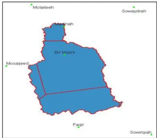
The study area is located within the upstream of Wadi Al-Aqiq in the Madinah province of the KSA (Figure 1). This region is mostly hilly with gentle and steeply sloping plains and barren rocks void of significant vegetative growth. In the study area, there are six sub-catchments including the upper portion of Wadi Al-Aqiq (4,839 km2_{), but the main area of concern in this study is the} area confined to about 400 km2 _{between latitude 24}o 28’ 55.8’’ N and longitude 39o _{33’ 2.5’’ E.}

The Madinah area is characterized by arid climate rainfall pattern with high temporal and spatial variability that takes place primarily during the winter and spring seasons [3, 5, 6]. The seasonal rainfall events are caused by the combination of disturbances from the winter Mediterranean and the Sudan trough, which usually generate extreme rainfall convective events over Madinah region and its surrounding areas [1, 6].

Figure 1 The study area in Wadi Al-Aqiq, Madinah

Since 1960, the Ministry of Agriculture and Water, now the Ministry of Water and Electricity (MoWE), Saudi Arabia, has established a hydrological network over different parts of the KSA, including Wadi Al-Aqiq in Madinah region. The Wadi network consists of meteorological stations in Wadi Al-Aqiq basin, which party covers Madinah City.

Figure 2 shows the Wadi Al-Aqiq catchment representation with the Theissen polygon. Seven stations make up the Wadi metrological/rainfall collection network, which are Bir Uthman, Madinah (M001), Bir Mashi (M103), Faqir (J109), Mosaijeed (J118), Molaileeh (M108), Sowaydrah (W109), and Sowirqiah (M110). The effective portion for individual stations within Wadi Al-Aqiq are M103 (56.72 %); J109 (30.96 %); M001 (6.22 %); MJ118 (5.91 %). Stations M110, W109, M108 have negligible areal percentage.

Figure 2 Thiessen polygon for rainfall distribution of Wadi Al-Aqiq catchment

1.2 Modeling Procedure

The historical rainfall statistics on annual and monthly basis for these stations are presented in Table 1.

Table 1 Major rainfall stations in the study area

Table 2 Summary of statistics of the monthly rainfall data sets

It can be observed from Table 2 that for all the records, the standard deviations are greater than their corresponding mean values with high values for skewness and kurtosis. The skewness indicates that the distribution is concentrated to the right, that is to say the distribution of the rainfall is left-skewed. The positive kurtosis shows a leptokurtic condition, with a fatter tail than normal, which indicates that the rainfall fluctuates through time [13, 14].

Assessment of climate change impact can be made by studying historical records of rainfall records.

1.3 Description of the Data Used

Sets of annual and monthly rainfall data for 4 stations in the KSA with different record lengths are used. The geographical coordinates of the registered stations and summary of statistics of the monthly rainfall data sets are given in Table 1 and 2 respectively.

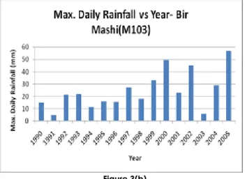
Figures 3a and 3b show the yearly maximum daily rainfall for M001 from 1980 to 1995 and M103 from 1990 to 2005, respectively.

Figure 3(a)

Figure 3(b)

Madinah station records have 2 peaks at around 85.2 mm and 89.6 mm in 1982 and 1993, respectively, while Bir Mashi has 3 peaks with about 49.5 mm, 45 mm, and 57 mm in 2000, 2002, and 2005, respectively. In 1993 Madinah station location was wetter with 85.2 mm of rainfall compared to Bir Mashi where only 22 mm was recorded.

Figure 3(c)

Figure 3(d) Station

Name Station ID Longitude (o_E)

Latitude (o_N) Type of data Record length (year) Madinah M001 39.58 24.49 Rainfall 43 Mosaijeed J118 39.08 24.08 Rainfall 48 Bir Mashi M103 39.58 24.18 Rainfall 44 Sowirqiah M110 40.32 23.34 Rainfall 46

Station name Period Mean Std. dev Skewness Kurtosis Sowirqiah 2004 – 2011 5.07 11.58 2.43 4.78 Bir Mashi 1989 – 2011 3.85 10.03 3.73 16.51 Mosaijeed 1999 – 2011 4.29 13.69 5.18 31.23 Madinah 1972 – 2011 3.86 11.05 5.56 43.37

Figures 3c and 3d compare the number of rainy days in Madinah and Bir Mashi. For instance, in 1993, Madinah station location had a maximum of 21 rainy days compared to 8 rainy days in Bir Mashi. This was due to two reasons; the distance factor (Madinah and Bir Mashi are 33 km apart) and the geographical features. The latter is more acceptable basis to explain the phenomena rather than distance as shown in the areal rainfall coverage of the Theissen polygons (see Figure 2).

Figure 3(e)

Figure 3(f)

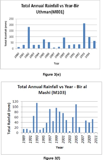
Figure 3 Time Series Plot of Annual Rainfall

Rainfall in Figure 3e and 3f provides comparison of the annual rainfall from 1990 to 2005 in Madinah and Bir Mashi stations. Figure 3e shows that Madinah has the highest total annual rainfall in 1982 and 1993with 183.2 mm and 212.3 mm, respectively. It can be seen from Figure 3f that Bir Mashi station received the highest annual rainfall as 114 mm and 109 mm in 1993 and 2005, respectively. Comparison of these figures for 1993 indicates that Madinah (M001) annual rainfall is two-fold higher than Bir Mashi station.

Forty-five years of seasonal records for (M001) are analyzed for the maximum daily rainfall and total annual rainy days, and the results are presented in

Figures 3a and 3c, respectively. Although very rare, two extremely high daily rainfalls are observed in years 1982 (88.2 mm) and 1993 (89.6 mm). These events have contributed to the maximum annual rainfall amounts. They have magnitudes that represent the rainfall depth experienced recently in Jeddah City, where on 26 November, 2009 96 mm of rainfall occurred leading to major flood damages. Meanwhile, Figures 3b and 3d are for 2000, 2002 and 2005 and they show the highest daily rainfall amounts at Bir Mashi (M103), which are 49.5 mm, 45 mm and 57 mm, respectively. Comparison of these figures for 1993 for Madinah shows that the highest daily rainfall was 89.2 mm

2.0 METHODOLOGY

2.1 Trend Detection Method

The Mann-Kendall M-K test trend test is a nonparametric and highly recommended by the World Meteorological Organization due to two advantages. It is not necessary that the data should be distributed according to the normal probability distribution and it has low sensitivity to abrupt break due to inhomogeneous time series [15]. The test hypothesis test states that there is no trend in the records and the alternative hypothesis is that there is significant trend [16].

In the null hypothesis, a series of independently and identically distributed random variables come from a population. The M-K test statistic is defined as,

(1) where,

,

On the other hand, Kendall’s measures the strength of the monotonic trend according to,

(2)

Kendall [17] showed that the variance of S, Var(S), for the situation where there may be ties (i.e., equal values) in the x values, is given by,

(3) where ‘m’ is the number of tied groups in the data set

and 𝑡𝑖 is the number of data points in the i-th tied group.

The Seasonal-Mann-Kendall (S-M-K) trend test is for monotonic trends in a time series with seasonal variations. Hirsch [18] developed a test by computing the Kendall score separately for each month. The separate monthly scores are then summed to obtain the test statistics. The variance of the test statistics is

1, 2,..., n x x x 1 0 ( ) 0 0 1 0 j i j i j i j i if x x sign x x if x x if x x            





 

obtained by summing the variances of the Kendall score statistics for each month. The normal PDF approximation may then be used to evaluate the significance level. The test null hypothesis is that the time series is of significant level of the form

, where is white noise error; represents the mean for period ‘m’; and coefficient is defined as,

(4) Note that and i = 1,…, s denote the Kendall scores and denominators for the i-th season; and s is the seasonal period

2.2 Detrended Fluctuation Analysis (DFA)

Before proceeding to modeling and forecasting aspect, there is need to investigate the scaling property of the data to see whether it is predictable. For this purpose, the Detrended Fluctuation Analysis (DFA) is used.

This is based on the classical root-mean square (RMS) analysis of a random walk. It is specifically designed to be less likely affected by non-stationarities. Consider a fluctuating time series , ( = 1, 2, . . , N), sampled at equidistant time intervals . One assumes that are increments of a random walk process around the average as,

(5) Thus the ‘‘trajectory’’ or ‘‘profile’’ of the signal is given by integration as:

(6) One can divide the profile into non-overlapping segments of equal lengths n indexed by k = [1, . . .,N/n]. In each segment, the local trend is fitted by a polynomial of order p, and the profile is de-trended by subtracting this local fit, as,

,

j = 1, . . ., N. (7) A possible measure of fluctuations can then be

given by the RMS for a given segment length n.

(8) A power-law relationship between and n

indicates scaling with an exponent (DFAp exponent): . Notice that such a process has a power-law autocorrelation function

, where 0 < α < 1. For α = 0.5, the series follows a white noise process with no prediction ability. For 0.5 < α < 1 and 0 < α < 0.5, the series has prediction ability.

2.3 State Space Exponential Smoothing Models

In most applications, there is a frequent need for fully automatic forecasting that takes into account trend, seasonality and other features of the data without need for human intervention. One of the most successful automatic forecasting methods in practice is based on exponential smoothing models implemented in the forecast package in r software. There are a variety of such models, each having the property that forecasts are weighted averages of past observations with recent observations given relatively more weight than older observations. The name “exponential smoothing” reflects the fact that the weights decrease exponentially as the observations get older. The exponential smoothing (ES) method is denoted by two letters: the first letter denotes the type of trend and the second letter denotes the type of seasonality component. A time series with no trend and seasonal components may not be suitable for this method.

2.3.1 Time Series Components

A time series is a stochastic procedure that describes the evolution of the random variable. Any random phenomenon that can be measured over time is a time series. A time series consist of four different components:

 Trend (T): A trend is a long-term component that represents a growth or a decline of a time series over an extended period of time.  Seasonal component (S): This term of

seasonality is used for time series defined at time intervals which are fractions of a year. It is a pattern of change that repeats itself from year to another.

 Cyclical component (C): Changes in time series sometimes show a wave-like fluctuation around a trend, which shows the possible existence of periodicity with longer intervals.  Irregular component (E): This is a part of a time

series represented by residuals, after the above-mentioned components have been removed. Any time series data that contained the above components is usually described using the following equation:

(9) The exponential smoothing always starts with the trend component, which is itself a combination of level term (l) and a growth term (b). The level and growth can be combined in different ways, given five future trend types. Let Th denote the forecast trend over the next h periods, and let ϕ denote a damping parameter (0 < ϕ < 1). Then the five trend types or growth patterns are as follows:

None: Th = l Additive: Th = l + bh t m t y 













0

x

N

x







y

x









Additive damped: Th = l + (ϕ + ϕ2 + …+ ϕh)b

Multiplicative: Th = lbh

Multiplicative damped: Th = lb(ϕ + ϕ2 + …+ ϕh)

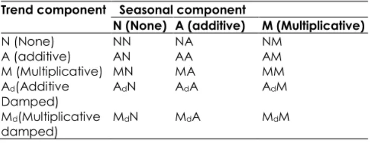
A damped trend method is appropriate when there is a trend in the time series. The equation for the damped trend dampens the trend as the length of the forecast horizon increases. Having chosen a trend component next is to introduce the seasonal component which is either additively or multiplicatively. Finally, in case of conclusion with an error component, either additively or multiplicatively, which are encapsulated within a state-space framework referred to as ETS for error (E), trend (T), and seasonal (S) components. Details can be found in Hyndman et al. [19]. If the error component is ignored, then one has the fifteen ES methods given in Table 3.

The models yield more realistic 95% prediction interval values. Furthermore, a reduction in the number of ES methods also reduces the expensive computational time. For more details of these models Hyndman [19] provides extensive explanations.

Table 3 Summary of 15 state space exponential smoothing models

Trend component Seasonal component

N (None) A (additive) M (Multiplicative)

N (None) NN NA NM A (additive) AN AA AM M (Multiplicative) MN MA MM Ad(Additive Damped) AdN AdA AdM Md(Multiplicative damped) M dN MdA MdM

The variables lt, bt and st are elements of the state

vector and denote the level, slope and seasonal components, respectively; the parameters α, β, and γ are the usual smoothing parameters corresponding to the level equation, trend equation and seasonal equation; ϕ is a damping coefficient used for the damped trend models; and m denotes the number of periods in the seasonal cycle. These three classes provide stochastic models for a wide variety of exponential smoothing methods.

Table 4 shows some ETS equations that generate point forecasts. The statistical models in this section generate the same point forecasts, but can also generate forecast intervals. Each model consists of a measurement equation that describes the observed data and some transition equations that describe how the unobserved components or states (level, trend, seasonal) change over time. Hence these are referred to as “state space models”.

Table 4 Some ETS State Space Exponential smoothing models equations Model Equation ANN 𝑦𝑡= 𝑙𝑡−1+ 𝜀𝑡 𝑙𝑡= 𝑙𝑡−1+ 𝛼𝜀𝑡 AAA 𝑦𝑡= 𝑙𝑡−1+ 𝑏𝑡−1+ 𝑠𝑡−𝑚+ 𝜀𝑡 𝑙𝑡= 𝑙𝑡−1+ 𝑏𝑡−1+ 𝛼𝜀𝑡 𝑏𝑡= 𝑏𝑡−1+ 𝛼𝛽𝜀𝑡 𝑠𝑡= 𝑠𝑡−𝑚+ 𝛾𝜀𝑡

Point forecasts are obtained from the models by iterating the equations for 𝑡 = 𝑇 + 1, 𝑇 + 2, … , 𝑇 + ℎ and setting all 𝜀𝑡= 0 for t > T. For example, for Artificial Neural Network (ANN) model, the observation equation is 𝑦𝑡= 𝑙𝑡−1+ 𝜀𝑡 and the state or level equation 𝑙𝑡= 𝑙𝑡−1+ 𝛼𝜀𝑡, where 𝜀𝑡= 𝑦𝑡+ 𝑙𝑡−1 = 𝑦𝑡+ 𝑦̂𝑡/𝑡−1 for 𝑡 = 1, 2, … , 𝑇, is sample forecast error at time t. 𝑙𝑡 is an unobserved state, therefore, must be estimated 𝛼 and 𝑙𝑡. For AAA models 𝑦𝑡= 𝑙𝑡−1+ 𝑏𝑡−1+ 𝑠𝑡−𝑚+ 𝜀𝑡 is the forecasting equation where 𝑙𝑡= 𝑙𝑡−1+ 𝑏𝑡−1+ 𝛼𝜀𝑡 level equation, 𝑏𝑡= 𝑏𝑡−1+ 𝛼𝛽𝜀𝑡 is the trend equation and 𝑠𝑡= 𝑠𝑡−𝑚+ 𝛾𝜀𝑡 is the seasonal equation. Therefore, 𝑙𝑡 , γ, s and 𝛽 need to be estimated.

2.4 ETS Models Diagnostic Checking

When a model for the data generating process of a time series has been constructed, it is a common practice to perform checks on the model adequacy. Tests for residual autocorrelation (AC) are prominent tools for this task. A well-known example is a Ljung-Box test for residual autocorrelation.

Checking for serial correlation for estimated residuals from a fitted model, which serves as a misspecification test for a linear dynamic regression model is necessary. The existence of serial correlation complicates statistical inference of time series analysis.

Ljung and Box proposed a Q-Test called Ljung–Box (LB) test which is commonly used in linear models. This test is applied to the residuals of a fitted model, not the original series, and in such applications the hypothesis to be tested is that the residuals from the model have no autocorrelation. A lack-of-fit hypothesis test for model misspecification based on the Q-statistic is given as:

(10) where N = sample size, L = number of autocorrelation lags included in the statistic, and is the squared sample autocorrelation at lag j. Under the null hypothesis of no serial correlation, the Q-test statistic is asymptotically Chi-Square distributed. The p-values above 0.05 indicate the acceptance of the null hypothesis of model accuracy under 95% significant levels (Wang et al. 2005).

2 1 ˆ ( 2) ( ) L j j Q N N N j     



ˆ



3.0 RESULTS AND DISCUSSION

3.1 Rainfall Trend Analysis

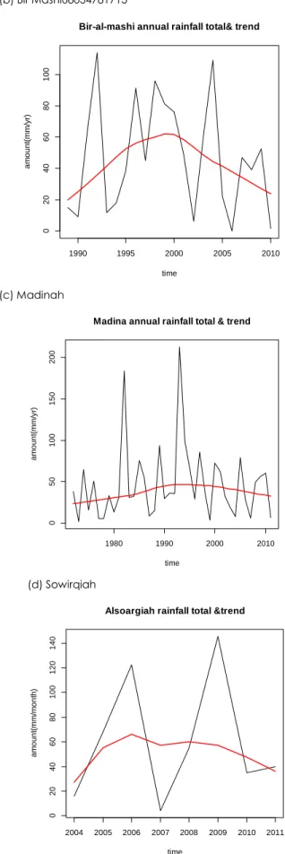
The magnitudes of the trends of increasing or decreasing annual rainfall and monthly rainfall totals were derived and tested by the Mann-Kendall (M-K) trend test. The non-parametric M-K statistical test was applied to determine whether long-term temporal trends exist for the meteorological stations. As mentioned in Section 4.1 the M-K test is a rank-based procedure that is less sensitive to outliers than parametric approaches, so it is widely used in hydrology and climatology. The magnitude of the trend is described by the M-K estimator at the confidence level at 95%. The seasonal M-K test takes into account the seasonality of the series. This means that the monthly data have a seasonality of 12 months. The test does not determine if there is a trend in the overall series, rather it takes into account whether a trend exists from one month to another, and so on. According to the positive or negative value of the tau-statistic for both level and seasonal trend test, the stations of Bir Mashi, Mosaijeed and Madinah present a decreasing long-term trend, while Sowirqiah show a slightly increasing trend (see Table 5).

The annual rainfall data(s) shows decreasing trend in all the stations (Figure 4). Decreasing rainfall would have negative impacts on water availability, which would in turn have an impact on different social and economic sectors [20].

(a) Almosijeed

(b) Bir Mashi08034781713

(c) Madinah

(d) Sowirqiah

Figure 4 (a-d) Time plot of annual rainfall total along with M-K trend line



Almosijeed annual rainfall total & trend

time a m o u n t( m m /yr ) 2000 2002 2004 2006 2008 2010 2012 0 20 40 60 80 100 120

Bir-al-mashi annual rainfall total& trend

time a m o u n t( m m /yr ) 1990 1995 2000 2005 2010 0 20 40 60 80 100

Madina annual rainfall total & trend

time a m o u n t( m m /yr ) 1980 1990 2000 2010 0 50 100 150 200

Alsoargiah rainfall total &trend

time a m o u n t( m m /m o n th ) 2004 2005 2006 2007 2008 2009 2010 2011 0 20 40 60 80 100 120 140

Table 5 Summary of results for the MannKendall and seasonal MannKendall tests

Station

name MannKendall Seasonal MannKendall

tau p-value tau p-value

Sowirqiah 0.0881 0.2669 0.0981 0.3276

Bir Mashi -0.0129 0.7828 -0.0141 0.7871 Mosaijeed -0.0861 0.1509 -0.1270 0.0746

Madinah -0.0403 0.2400 -0.0354 0.3229

3.2 De-Trended Fluctuation Analysis

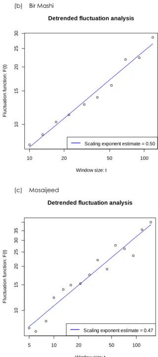
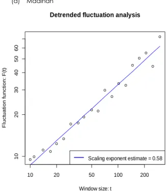
The de-trended fluctuation analysis (DFA) method has been proposed to quantify the complexity of a non-stationary time series. It is an important tool for the determination of fractal scaling properties and also for long-range correlations in noisy time series. In this study, the DFA method is applied to the time series of monthly rainfall totals of 4 respective stations in the KSA. Figures 5a-5d depict the fluctuation process and the scaling exponents using the DFA method.

(a) Sowirqiah (b) Bir Mashi (c) Mosaijeed



Detrended fluctuation analysis

Window size: t F lu ct u a ti o n f u n ct io n : F (t )

Scaling exponent estimate = 0.49

10 20 50 100 10 15 20 25 30

Detrended fluctuation analysis

Window size: t F lu ct u a ti o n f u n ct io n : F (t )

Scaling exponent estimate = 0.50

5 10 20 50 100 10 15 20 25 30 35

Detrended fluctuation analysis

Window size: t F lu ct u a ti o n f u n ct io n : F (t )

(d) Madinah

Figure 5 (a-d) De-trended fluctuation processes with estimate

The application of the DFA (Figure 5a-d) indicate that out of the four stations, only three (Mosaijeed, Sowirqiah and Bir Mashi) have scaling exponents as approximately 0.5. A scale exponent close to 0.5 is an indication that the rainfall fluctuations of all the three stations are characterized by a white noise process, which is a sequence of uncorrelated random variables that exhibit a very erratic, jumpy and unpredictable behaviour. Hence previous values do not help in forecasting future values.

The monthly rainfall time series observed at Madinah station has a scaling exponent of 0.58, which is indicative of a persistent behaviour. In a persistent time series an increase in values will most likely be followed by an increase in the short term and a decrease in values will most likely be followed by another decrease in the short-term. Hence, the observed rainfalls in Madinah station have a predictable component, and therefore, past observations could be used to predict the future. To evaluate the influence of this particular characteristic on the results of DFA, one can predict upcoming rainfall in the study areas.

3.3 ETS State Space Exponential Smoothing Modelling

Application of the automatic forecasting strategy to fish catch is to demonstrate that the methodology is particularly good at short term forecasts and especially for seasonal short-term series. This was achieved without any data pre-processing, or other strategy designed to improve the forecasts. In this case the data is decomposed to see whether its component will suit ETS modelling.

3.3.1 Time Series Components

Decomposition procedures are used in time series to describe the trend and seasonal factors in a time series. One should note that the seasonal pattern is a regularly repeating pattern. One of the main objectives for decomposition is to estimate seasonal effects that can be used to create and present seasonally adjusted values. A seasonally adjusted value removes the seasonal effect from a value so that trends can be seen more clearly.

The trend of a time series is considered as a smooth additive component that contains information about change in parameters. Over the years there has been an increasing concern on whether there is an increasing or decreasing trend in Wadi Al-Aqiq rainfall. The time series decomposition plots (Figure 6a-d) separate the series into its constituent components i.e., the estimated trend component (T), the random component (E) and the estimated seasonal component (S).

The plots show the estimated trend component and seasonal components also displayed in all the figures. These components observed in the rainfall data sets might be comfortable with the ETS state space exponential smoothing models.

a) Sowirqiah 10 20 50 100 200 10 20 30 40 50 60

Detrended fluctuation analysis

Window size: t F lu ct u a ti o n f u n ct io n : F (t )

Scaling exponent estimate = 0.58





b) Bir Mashi

c) Mosaijeed

d) Madinah

Figure 6 (a-d) Monthly rainfall time series decomposition plots

Exponential smoothing methods are useful for making forecasts, and require no assumptions about the correlations between successive values of the time series. The ETS models that adequately fit the data sets are described in Table 5. The parameters used in generating these models are also shown in the same table. These parameters are chosen to generate data that look reasonably realistic. Clearly, the algorithm has a very high success rate at determining whether the errors should be additive or multiplicative. Table 6 gives the parameters estimates of the fitted models for the stations considered.

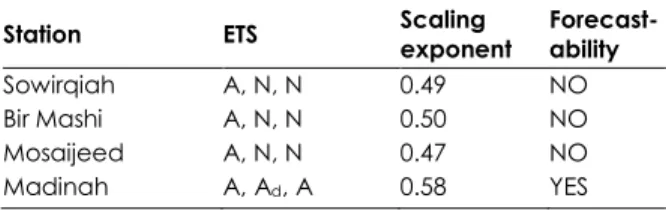
Table 5 Summary of results for ETS models and their forecast-ability

Station ETS Scaling _exponent Forecast-_ability

Sowirqiah A, N, N 0.49 NO

Bir Mashi A, N, N 0.50 NO

Mosaijeed A, N, N 0.47 NO

Madinah A, Ad, A 0.58 YES

Table 6 ETS models parameter estimates

Parameter s 𝒍

Sowirqiah 1e-04 - - 11.52 - - 5.06

Bir Mashi 1e-04 - - 10.02 - - 3.85

Mosaijeed 1e-04 - - 13.65 - - 4.32

Madinah 2e-04 2e-04 4e-04 10.62 0.81 1.02 -0.57

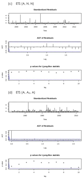
3.3.2 ETS Models Diagnostic Results

In order to be sure whether the fitted ETS models can be representative of the data sets and could be used to forecast the upcoming rainfall, one needs to test the models residuals against serial correlation. Figures 7a-d depicts the plot of the residual, ACF of residual and the LB test results. The results from Figures 7a-7d show that most autocorrelations of the residuals from the fitted ETS models are within the limits upon which the models are based. Therefore, the residuals are uncorrelated suggesting that the models are adequate to represent the data sets. The Ljung-Box test result also confirmed the evidence of no autocorrelations in the residuals, which is enough evidence to conclude that a model is adequate. This suggests that the ETS exponential smoothing methods provide adequate predictive models for the monthly rainfall total of the stations considered.

0 20 40 60 o b se rve d 0 2 4 6 8 10 tr e n d -4 -2 0 2 4 se a so n a l 0 20 40 60 1990 1995 2000 2005 2010 ra n d o m Time

Decomposition of additive time series

0 20 60 100 o b se rve d 0 2 4 6 8 10 tr e n d -5 0 5 10 se a so n a l -2 0 20 60 2000 2002 2004 2006 2008 2010 2012 ra n d o m Time

Decomposition of additive time series

0 40 80 120 o b se rve d 0 5 10 15 tr e n d -4 -2 0 2 4 se a so n a l -2 0 20 60 100 1980 1990 2000 2010 ra n d o m Time

Decomposition of additive time series

(a) ETS (A, N, N)

(b) ETS (A, N, N)

(c) ETS (A, N, N)

(d) ETS (A, Ad, A)

Figure 7 (a-d) Diagnostic plot of the fitted ETS models

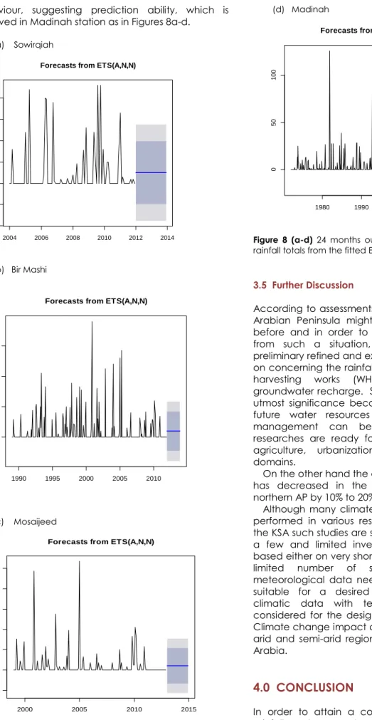
3.4 Rainfall Prediction with ETS Models

The ETS models have been presented to forecast 24 month rainfall in some locations in the KSA However, these models generally gives poor results for Sowirqiah, Mosaijeed and Bir Mashi stations as shown in Figure 8a, b and c. This result is not surprising as evidence has been in place that both series are uncorrelated and do not have prediction ability. Moreover, the rainfall in Madinah does have prediction ability as shown in Figure 8d. The DFA revealed two distinct scaling properties in the rainfall records. The first is observed in Mosaijeed, Bir Mashi and Sowirqiah with scaling exponents as approximately 0.5 suggesting non-predictive behaviour equally confirmed in the forecast plots in Figures 8b, c and d. The second is persistent

Standardized Residuals Time 2004 2006 2008 2010 2012 0 1 2 3 0.5 1.0 1.5 -0 .2 0 .0 0 .2 ACF of Residuals Lag A C F 2 4 6 8 10 0 .0 0 .4 0 .8

p values for Ljung-Box statistic

lag p v a lu e Standardized Residuals Time 1990 1995 2000 2005 2010 0 2 4 6 0.5 1.0 1.5 2.0 -0 .1 0 0 .0 5 ACF of Residuals Lag A C F 2 4 6 8 10 0 .0 0 .4 0 .8

p values for Ljung-Box statistic

lag p v a lu e Standardized Residuals Time 2000 2002 2004 2006 2008 2010 2012 0 2 4 6 0.5 1.0 1.5 -0 .1 5 0 .0 0 0 .1 5 ACF of Residuals Lag A C F 2 4 6 8 10 0 .0 0 .4 0 .8

p values for Ljung-Box statistic

lag p v a lu e Standardized Residuals Time 1980 1990 2000 2010 0 4 8 0.0 0.5 1.0 1.5 2.0 0 .0 0 .4 0 .8 Lag A C F ACF of Residuals 2 4 6 8 10 0 .0 0 .4 0 .8

p values for Ljung-Box statistic

lag p v a lu e

behaviour, suggesting prediction ability, which is observed in Madinah station as in Figures 8a-d.

(a) Sowirqiah

(b) Bir Mashi

(c) Mosaijeed

(d) Madinah

Figure 8 (a-d) 24 months out sample prediction of monthly rainfall totals from the fitted ETS models

3.5 Further Discussion

According to assessments of the IPCC [21] report, the Arabian Peninsula might receive more rainfall than before and in order to have the maximum benefit from such a situation, it is necessary to make preliminary refined and extensive researches from now on concerning the rainfall pattern coupled with water harvesting works (WH) possibilities leading to groundwater recharge. Such works are considered of utmost significance because near and long fetching future water resources planning, operation, and management can be successful only if such researches are ready for applications in hydrology, agriculture, urbanization, land use, and similar domains.

On the other hand the annual average precipitation has decreased in the Mediterranean region and northern AP by 10% to 20%, respectively.

Although many climate change studies have been performed in various research centres worldwide, in the KSA such studies are still in their infancy where only a few and limited investigations have been done based either on very short periods by using only a very limited number of surface stations Available meteorological data need to be analyzed in a way suitable for a desired application. For instance, climatic data with temporal variation can be considered for the design of water resources system. Climate change impact can prove more critical in the arid and semi-arid regions like The Kingdom of Saudi Arabia.

4.0 CONCLUSION

In order to attain a comprehensive picture of the rainfall, we have analysed the annual monthly rainfall Forecasts from ETS(A,N,N)

2004 2006 2008 2010 2012 2014 -2 0 -1 0 0 10 20 30 40

Forecasts from ETS(A,N,N)

1990 1995 2000 2005 2010

0

20

40

60

Forecasts from ETS(A,N,N)

2000 2005 2010 2015 -2 0 0 20 40 60 80 100

Forecasts from ETS(A,Ad,A)

1980 1990 2000 2010

0

50

records of four weather stations around the Wadi Al-Aqiq. We have studied the annual and monthly rainfall trends and forecast ability for all the four stations’ rainfall records namely: Sowirqiah, Mosaijeed, Bir Mashi and Madinah, separately. The annual and monthly rainfall shows decreasing trends in all the observed records excluding Sowirqiah station which exhibits a gradual increase in trend. This is confirmed by Mann-Kendall trend test.

The de-trended fluctuation analysis revealed two distinct scaling properties in the rainfall records. The first is observed in Mosaijeed, Bir Mashi and Sowirqiah and the second is persistent behaviour, suggesting prediction ability which is observed in Madinah station. The points indicate the types of information expected as relevant to water resources of the KSA, in particular, and of the arid and semi-arid regions, in general.

Acknowledgement

This study was supported by the National Plan for Science, Technology and Innovation (MAARIFAH) – King Abdulaziz City for Science and Technology – the Kingdom of Saudi Arabia, award number 10-WAT1049-05 and Science and Technology Unit at Taibah University, Madinah, Saudi Arabia. The authors express their thanks to the Ministry of Water and Electricity (MoWE), Saudi Arabia for providing the rainfall data. Also, the authors would like to thank the Research Management Centre (RMC) of Universiti Teknologi Malaysia (UTM) for their grant support in conducting this research (PY/2017/00598).

References

[1] Subyani, A. M., Al-Ahmadi, F. S. 2011. Rainfall-runoff modeling in the Almadinah area of Western Saudi Arabia.

Journal of Environmental Hydrology. 19(1).

[2] Abd Rahman, N., Taher, S., Alahmadi, F. and Mohd Nasir, K. A. 2016. Arid Hydrological Modeling at Wadi Alaqiq, Madinah, Saudi Arabia. Jurnal Teknologi. 78: 7.

[3] Subyani, A. M., Al-Modayan, A. A. and Al-Ahmadi, F. S. 2010. Topographic, Seasonal And Aridity Influences On Rainfall Variability In Western Saudi Arabia. Journal of Environmental

Hydrology. 18(2).

[4] Alahmadi, F., Abd Rahman, N. and Abdulrazzak, M. 2014. Evaluation Of The Best Fit Distribution For Partial Duration Series Of Daily Rainfall In Madinah, West Of Saudi Arabia, Evolving Water Resources System: Understanding, Predicting

and Managing Water-Society Interactions. Proceedings of

ICWRS 2014, Bologna, Italy. IAHS Publ. 364.

[5] Alahmadi, F., Abd Rahman, N. and Yusop, Z. 2016. Hydrological Modeling Of Ungauged Arid Volcanic Environments At Upper Bathan Catchment, Madinah, Saudi Arabia. Jurnal Teknologi. 78: 9-4.

[6] Abd Rahman, N., Alahamdi, F., Sen, Z. and Taher, S. 2016. Frequency Analysis Of Annual Maximum Daily Rainfall In Wadi Alaqiq, Saudi Arabia. Malaysian Journal of Civil

Engineering. 28(2): 237-256.

[7] Almazroui, M., Nazrul Islam, M., Jones, P. D., Athar, H. and Ashfaqur, M. R. 2012. Recent Climate Change In The Arabian Peninsula: Seasonal Rainfall And Temperature Climatology Of Saudi Arabia For 1979–2009. Atmospheric

Research. 111: 29-45.

[8] Trigo R. M., Pozo-va´zquez, D., Osborn, T. J., Castro-Di´ez. Y., Ga´mız-Fortis, S., and Esteban-Parra, M. J. 2004. North Atlantic Oscillation Influence On Precipitation, River Flow And Water Resources In The Iberian Peninsula. International

Journal Climatology. 24: 925-944.

[9] Jones, P. D., Moberg, A. 2003. Hemispheric And Large-Scale Surface Air Temperature Variations: An Extensive Revision And An Update To 2001. Journal Climate. 16: 206-223, [10] Şen, Z., Al-Alsheikh, A., Al-Dakheel, A. M., Alamoud, A. I.,

Alhamid, A. A, El-Sebaay, A. S., Abu-Risheh, A. W. 2011a. Climate Change Impact And Water Harvesting Possibilities In Arid Regions: A Review. International Journal Global

Warming. 3(4):355-371.

[11] Şen, Z., Alsheikh, A., Turbak, A. S., Bassam, A.M., Al-Dakheel, A. M. 2011b. Climate Change Impact And Runoff Harvesting In Arid Regions. Arabian Journal of Geosciences. DOI:10.1007/s12517-011-0354-z.

[12] Şen, Z. 2012. Innovative Trend Analysis Methodology. Journal

Hydrology Engineering. 17(9): 1042-1046.

[13] Yusof, F. and Kane, I. L. 2012. Modeling Monthly Rainfall Time Series Using Ets State Space And Sarima Models.

International Journal of Current Research. 4(9): 195-200.

[14] Yusof, F., Kane, I. L. and Yusop, Z. 2013. Structural Break Or Long Memory: An Empirical Survey On Daily Rainfall Data Sets Across Malaysia. Hydrol. Earth Syst. Sci. 17: 1311-1318. [15] Tabari, H., Talaee, P. H. 2011. Temporal Variability Of

Precipitation Over Iran: 1966-2005. Journal of Hydrology. 396: 3-4, 313-320.

[16] Chaouche, K., Neppel, L., Dieulin, C., et al. 2010. Analyses Of Precipitation, Temperature And Evapotranspiration In A French Mediterranean Region In The Context Of Climate Change. Comptes Rendus Geoscience. 342: 3, 234-243. [17] Kendall, M. G. 1975. Rank Correlation Methods. Oxford Univ.

Press, New York.

[18] Hirsch, R. M., Slack, J. R. and Smith, R. A. 1982. Techniques for trend assessment for monthly water quality data. Water

Resources Research. 18: 107-121.

[19] Hyndman, R. J. and Khandakar, Y. 2008. Automatic the forecasting package for R. Journal of Statistical Software. www.jstatsoft.org .

[20] Ghanem, A. A. 2013. Case Study: Trends and Early Prediction of Rainfall in Jordan. American Journal of

Climate Change. 2: 203-208.

[21] IPCC Report. 2007. The Fourth Assessment Report (AR4). http:/www.ippc.ch/, March 14, 2008.