IS S N 1 3 0 3 –5 9 9 1
INVESTIGATION OF TREND BY GRAPHICAL METHODS IN COUNTING PROCESSES
MUSTAFA H·ILM·I PEKALP, HAL·IL AYDO ¼GDU AND ·IHSAN KARABULUT
Abstract. A data set fX1; X2; :::; Xng comes from a counting process
in many of maintenance, repair and replacement problems commonly includes systematical changes. Systematical changes in the data set indicate a trend which suggests thatX1; X2; :::; Xn are not identically
distributed. In this case renewal process cannot be used as a model. In modelling of a data set the existence of a trend has to be searched …rstly. A simple way to detect a trend is to apply a graphical method. In this study the cumulative number of failures versus the cumulative time plot, estimating the rate of occurrence of failures in successive time periods plot, Nelson-Aalen plot and the total time on test plot will be described and evaluated on three real data sets.
1. INTRODUCTION
Let (Xk)k=1;2;:::be a sequence of nonnegative random variables representing the
successive lifetimes. De…ne, S0= 0; Sk =
Pk
j=1Xj; k = 1; 2; : : : and
N (t) = supfk : Sk tg; t 0: The stochastic process fN(t); t 0g is called a
counting process. The (Xk)k=1;2;::: and Sk are often called the interarrival times
and kth arrival time, respectively.
A reasonable model should re‡ect the nature of the data at the hand. Hence, it is important to detect possible systematic changes in a data set observed from a counting process. The purpose of this study is to present some graphical methods to identify the trend in the data with systematical changes.
A data set fX1; X2; :::; Xng comes from a counting process includes systematic
changes frequently. A trend in the data set fX1; X2; :::; Xng indicates that the
random variables X1; X2; :::; Xn are not identically distributed. A trend in the
data can be either monotonic or non-monotonic. Monotonic trend denotes that intrearrival times tend to get longer (decreasing trend or improving system) or
Received by the editors May 23, 2014, Accepted: June 08, 2014. 2000 Mathematics Subject Classi…cation. 60K05, 62G05, 62-09.
Key words and phrases. Nelson-Aalen plot, NHPP, Renewal process, ROCOF, Trend, TTT plot.
c 2 0 1 4 A n ka ra U n ive rsity
shorter (increasing trend or deteriorating system). In the case of a non-monotonic trend it can be cyclic or bathtube trend. The most common types of trend in applications are monotone trend and bathtube trend.
If there is no trend in the data a renewal process can be used as a model. In particular, if the interarrival times are independent and identically distributed (iid) having exponential distribution, one must use a homogeneous Poisson process. If there is a trend in the data, a non-homogeneous Poisson process or a stochastic monotone process can be used.
A simple informative way is to apply graphical methods for visual examination and quali…cation of a data set coming from a counting process. In general, the data without trend will come up with a pattern which has spread around a linear straight line. The deviation from linearity will lead to doubt that there is a trend. There are some graphical methods to detect the trend and its nature.
2. SOME COUNTING PROCESSES
Failure times of a system are usually modelled by a counting process. In this section, the most common stochastic models will be reminded.
Renewal process. Let fN(t); t 0g be a counting process. If the interarrival times X1; X2; ::: are iid with a distribution function F , the counting process
fN(t); t 0g is called a renewal process (RP).
Homogeneous Poisson process. A counting process fN(t); t 0g is said to be a homogeneous Poisson process (HPP) having rate , > 0, if the process satis…es the following conditions. (1) N (0) = 0, (2) fN(t); t 0g has independent and stationary increments, (3) P (N (h) = 1) = h + o(h), (4) P (N (h) 2) = o(h).
According to a HPP the interarrival times X1; X2; ::: are independent and
iden-tically exponential distributed with mean 1= . Hence, HPP is a special RP. Non-homogeneous Poisson process. Let fN(t); t 0g be a counting process and
(t) is a function of t for t 0. If fN(t); t 0g satis…es the following conditions, it is called a non-homogeneous Poisson process (NHPP) with intensity function (t). (1) N (0) = 0, (2) fN(t); t 0g has independent increments,
(3) P (N (t + h) N (t) = 1) = (t)h + o(h), (4) P (N (t + h) N (t) 2) = o(h) Let fN(t); t 0g be a NHPP with intensity function (t). Then,
N (t + s) N (s) Poisson (M (t + s) M (s)), where M (t) =R0t (s)ds [7]. Thus, N (t) has Poisson distribution with mean M (t) for all t > 0.
The most common types of (t) are powerlaw and loglinear functions [2]. These are given as (t) = t( 1); t 0 ; ; > 0 and (t) = e + t ; t 0 ; ; 2 R, respectively.
The NHPP with constant intensity (t) = is a HPP with intensity .
Geometric process. Let fN(t); t 0g be a counting process. The fN(t); t 0g is said to be a geometric process (GP) with ratio parameter a if there exists a real
number a > 0 such that Yi = ai 1Xi, i = 1; 2; : : : are iid random variables with
distribution function F .
It can be easily shown that GP is stochastically increasing if 0 < a < 1 and stochastically decreasing if a > 1. If a = 1, GP reduces to a RP [3].
3. GRAPHICAL METHODS
In the literature there are many graphical methods to detect the presence of trend and its nature. Some of them are given below.
3.1. Cumulative number of failures versus cumulative time plot. The interarrival times tend to become larger (smaller) when the structure of a system is improving (deteriorating). Thus plotting the cumulative number of failure versus cumulative time will tend to be concave (convex) for improving (deteriorating) system.
3.2. Estimating ROCOF in successive time periods plot. Local variations will tend to be hidden because of the monotonically increasing nature of cumulative failures. In this situation, an alternative method is to divide the total observation interval into three or more subintervals and to estimate the rate of occurrence of failures (ROCOF) for all subintervals. If the system is improving (deteriorating) the estimates of ROCOF in successive time periods will tend to be decreasing (increasing).
Let fN(t); t 0g be a counting process. The expected value of N(t) is de…ned by M (t), that is, M (t) = E(N (t)). It is assumed that M (t) is absolutely continuous. Then, ROCOF is de…ned by (t) = dM (t)dt . The ROCOF has the following simple interpretation: (t) t is the probability that a failure, not necessarily the …rst, occurs in (t; t + t][1].
Assume that a data set fX1; X2; :::; Xng comes from a counting process
fN(t); t 0g. Since (t) = dM (t)dt , a natural estimator of (t) with an appropriate
t is as follows.
^(t) = 1 t
Pn
i=1I(t < X1+ X2+ ::: + Xi< t + t) (3.1)
where I(:) is an indicator function and the summation in (3.1) denotes the number of the failures in the interval (t; t + t] based on the data set fX1; X2; :::; Xng.
If the total observation interval (0; Sn] is divided into k subinterval as (0; a1];
(a1; a2]; : : : ; (ak 1; ak], an estimator of (12(aj 1+ aj)) for j = 1; 2; : : : ; k is
^(1
2(aj 1+ aj))=N (aajj) N (aaj 1j 1) [1].
Thus, it can be reached that a plot of ^(bj) versus bj where bj = 12(aj 1+ aj),
j = 1; 2; : : : ; k. This plot will give a plausible evidence for the shape of intensity (t).
3.3. Nelson-Aalen plot. Assume that m systems are observed and the processes related to systems will be independent and identical with probability one. Suppose further that the kth process is observed on the time interval (0; k] and let y(t)
denote the number of the processes under observation or running at time t. It is clear that y(t) =Pmk=1I( k t).
For t 0, let us write N (t) =Pmk=1Nk(t), where fNk(t); t 0g, k = 1; 2 : : : ; m,
is the individual failure process. The counting process fN(t); t 0g is called a superposed process. Let Sk denote the kth arrival time in the superposed process,
hence 0 < S1 SN , where N = N ( ) and = maxf k : k = 1; : : : ; mg.
De…ne the mean value function of a single failure process to be M (t) = E(N1(t)).
M (t) has a nonparametric Nelson-Aalen estimator as ^M (t) = PSk ty(S1
k). Thus
the plot of this estimator versus cumulative time is called Nelson-Aalen plot [4]. The deviation from linearity in this plot will lead to doubt that there is a trend. 3.4. TTT plot. Assume that m systems are observed and the processes related to systems will be independent and identical NHPP with a common intensity function (t). For each t 0, y(t) =Pmk=1I( k t) is the number of the processes under
observation at time t, where k; k = 1; : : : ; m, is the observation period for the kth
failure process fNk(t); t 0g. It is clear that the function y(t) is independent from
the kth arrival time Sk of the superposed process fN(t); t 0g. Since the failure
processes fN1(t); t 0g; : : : ; fNm(t); t 0g are independent NHPP with the same
intensity function (t), the superposed process fN(t); t 0g will be a NHPP with intensity function (t) = y(t) (t).
De…ning the total time on test (TTT) as r(t) =R0ty(u)du, the TTT plot is given by the points (Nk;r(Sk)
r( )) k = 1; : : : ; N where N = N ( ), that is, N is the total
number of failures in the time interval (0; ] [4]. It is obvious that r( ) =Pmk=1 k.
The TTT plot will be located near the main diagonal line on the unit square if there is no trend in the data set, that is, (t) is a constant. Under the alternatives of decreasing, increasing and bathtube shaped intensity (t), the TTT plot appears to be convex, concave and S-shaped, respectively.
4. APPLICATIONS OF THE GRAPHICAL METHODS ON THREE REAL DATA SETS
In this section, the graphical methods will be evaluated by using three real data sets.
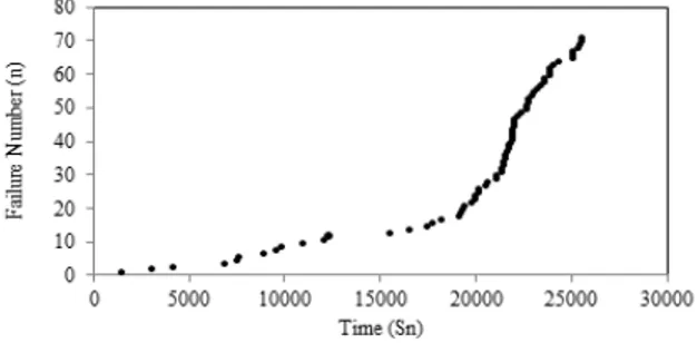
Example 4.1. The cumulative failure times in operating hours to unscheduled maintenance actions for the USS Halfbeak No.3 main propulsion diesel engine are given in the following Table 4.1 [1]. It is assumed that the system was observed until the 71st failure at 25518 hours.
Table 4.1. Cumulative failure times to unscheduled maintenance actions for the USS Halfbeak No.3 main propulsion diesel engine [1]:
1382 17632 21309 21943 23791 2990 18122 21310 21946 23822 4124 19067 21378 22181 24006 6827 19172 21391 22311 24286 7472 19299 21456 22634 25000 7567 19360 21461 22635 25010 8845 19686 21603 22669 25048 9450 19940 21658 22691 25268 9794 19944 21688 22846 25400 10848 20121 21750 22947 25500 11993 20132 21815 23149 25518 12300 20431 21820 23305 15413 20525 21822 23491 16497 21057 21888 23526 17352 21061 21930 23774
The cumulative number of failures versus the cumulative time is plotted in Figure 4.1. It is fairly apparent that the plot is convex. Thus, the data show very strong evidence for increasing trend.
Figure 4.1. Cumulative failures versus cumulative times for unscheduled maintenance actions for the USS Halfbeak No.3 main propulsion diesel engine.
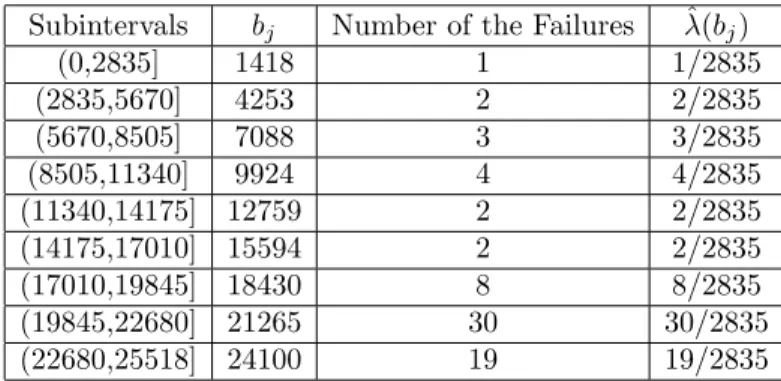
The estimates of ROCOF (t) are presented in Table 4.2 by taking t = 2835 (or 9 subintervals) for USS Halfbeak No.3 main propulsion diesel engine data.
Table 4.2. Number of the failures for unscheduled maintenance actions for the USS Halfbeak No.3 main propulsion diesel engine
and estimated (t) values
Subintervals bj Number of the Failures ^(bj)
(0,2835] 1418 1 1/2835 (2835,5670] 4253 2 2/2835 (5670,8505] 7088 3 3/2835 (8505,11340] 9924 4 4/2835 (11340,14175] 12759 2 2/2835 (14175,17010] 15594 2 2/2835 (17010,19845] 18430 8 8/2835 (19845,22680] 21265 30 30/2835 (22680,25518] 24100 19 19/2835
The illustration of ^(t) calculated in Table 4.2 is given by Figure 4.2.
Figure 4.2. Plot of 2835 times the estimated ROCOF against time for unscheduled maintenance actions for the USS Halfbeak No.3 main propulsion diesel engine
data.
Looking at the Figure 4.2, the USS Halfbeak No.3 main propulsion diesel engine data show apparent evidence for trend as revealed by cumulative failures versus cumulative times plot in Figure 4.1.
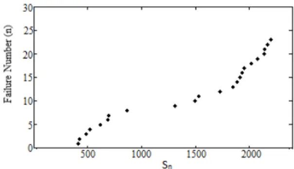
Example 4.2. The interarrival times in operating hours between the failures for a Boeing 720 aircraft ventilation system are given in the following Table 4.3 [6].
Table 4.3. Interarrival times between the failures for a Boeing 720 aircraft ventilation system.
413 9 118 57 14 169 34 62 58 447 31 7 37 184 18 22 100 36 18 34 65 201 67
At …rst glance, it can easily be seen that towards the end the failures tend to become more frequent. This brings to mind the idea that there is a trend in the data set fX1; X2; : : : ; X23g so these random variables are not identically distributed.
The cumulative number of failures versus the cumulative time is plotted in Figure 4.3.
Figure 4.3. Cumulative failures versus cumulative times for a Boeing 720 aircraft ventilation system.
From Figure 4.3 it can be concluded that there is a non-monotonic trend in the data.
The estimates of ROCOF (t) are presented in Table 4.4 by taking t = 440 (or 5 subintervals) for a Boeing 720 aircraft ventilation system data.
Table 4.4. Number of the failures for a Boeing 720 aircraft ventilation system data and estimated (t) values.
Subintervals bj Number of the Failures ^(bj)
(0,440] 220 2 2/440
(440,880] 660 6 6/440
(880,1320] 1100 1 1/440
(1320,1760] 1540 3 3/440
(1760,2201] 1980.5 11 11/440
Figure 4.4. Plot of 440 times the estimated ROCOF against time for the Boeing 720 aircraft data.
In Figure 4.4, it is clear that there is a trend in the pattern of the failures, and also the shape of the trend is non-monotonic. Thus, two graphical methods give us the same conclusion for trend with this data set.
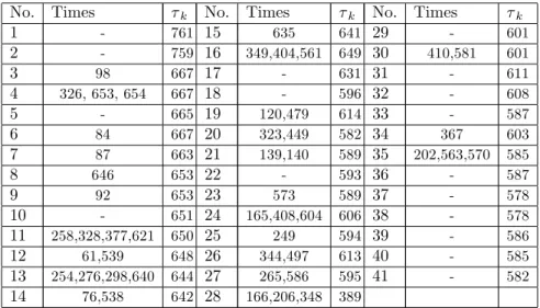
Example 4.3. The valve-seat replacement times for 41 diesel engines are given in Table 4.5 [5].
Table 4.5. Valve-seat replacement times in days for 41 diesel engines.
No. Times k No. Times k No. Times k
1 - 761 15 635 641 29 - 601 2 - 759 16 349,404,561 649 30 410,581 601 3 98 667 17 - 631 31 - 611 4 326, 653, 654 667 18 - 596 32 - 608 5 - 665 19 120,479 614 33 - 587 6 84 667 20 323,449 582 34 367 603 7 87 663 21 139,140 589 35 202,563,570 585 8 646 653 22 - 593 36 - 587 9 92 653 23 573 589 37 - 578 10 - 651 24 165,408,604 606 38 - 578 11 258,328,377,621 650 25 249 594 39 - 586 12 61,539 648 26 344,497 613 40 - 585 13 254,276,298,640 644 27 265,586 595 41 - 582 14 76,538 642 28 166,206,348 389
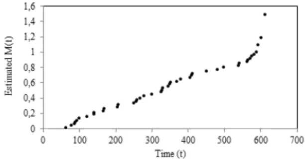
The values of ^M (t) are meaningful for t , since ^M (t) is constant for t > and, thus, meaningless. The following …gure is drawn by using the calculated nonparametric estimates of M (t) for the valve-seat data set. As an example, the value of ^M (t) is 0:15 for t = 98.
Figure 4.5. Nelson-Aalen plot.
In Figure 4.5, the ROCOF can be considered to be constant for the …rst 550 days, and then increases as revealed from the convex shape of the plot at the right end. Thus, it can be said that the data exhibit a trend.
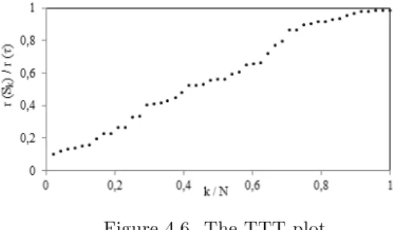
Let us consider again the valve-seat replacement data set. Using the calculated values given in Table 4.6, the TTT plot is displayed in Figure 4.6.
Table 4.6. The values of (Nk; r(Sk)
r( )) in TTT plot with N = 48 and k = 1; : : : ; 48: k N r(Sk) r( ) k N r(Sk) r( ) k N r(Sk) r( ) 0,0208 0,0986 0,3541 0,4283 0,6875 0,7991 0,0416 0,1228 0,375 0,4461 0,7083 0,8638 0,0625 0,1357 0,3958 0,4817 0,7291 0,8653 0,0833 0,1406 0,4166 0,5221 0,75 0,9 0,1041 0,1487 0,4375 0,5269 0,7708 0,9032 0,125 0,1584 0,4583 0,5302 0,7916 0,9142 0,1458 0,1939 0,4791 0,556 0,8125 0,919 0,1666 0,2246 0,5 0,5625 0,8333 0,9313 0,1875 0,2263 0,5208 0,5641 0,8541 0,9384 0,2083 0,2667 0,5416 0,5932 0,875 0,9576 0,2291 0,2683 0,5625 0,6094 0,8958 0,9702 0,25 0,3265 0,5833 0,6524 0,9166 0,9794 0,2708 0,333 0,6041 0,6587 0,9375 0,9826 0,2916 0,4025 0,625 0,6619 0,9583 0,986 0,3125 0,4105 0,6458 0,7234 0,9791 0,989 0,3333 0,417 0,6666 0,7707 1 0,9893
Figure 4.6. The TTT plot.
The TTT plot in Figure 4.6 shows that the ROCOF is fairly constant, but it increases with a slightly concave shape near the end. Hence it can be concluded that the data have a trend as revealed by the Nelson-Aalen plot in Figure 4.5.
5. DISCUSSION
In this paper, some of graphical methods are reviewed to detect the presence of trend and its nature. The plot of cumulative failures versus cumulative time is simple to apply. Nevertheless, local variations will tend to be hidden because of the monotonically increasing nature of cumulative number of failures. An alternative method is to plot of estimated ROCOF [1]. However, this method is sensitive for selected values of k and aj. Some di¤erent inferences can be obtained based on the
selection of k or aj. The choice of k or aj is similar to the choice of the number
of intervals or the interval width for a histogram. The Nelson-Aalen plot can be considered as a generalization of the plot of cumulative failures versus cumulative times. When m equals to 1 the Nelson-Aalen plot is a plot of cumulative failures versus cumulative times. The TTT plot is often used to test whether the counting process fN(t); t 0g is a HPP with = 1, as well as to detect trend in the data set fX1; X2; : : : ; Xng [4].
References
[1] Ascher, H. and Feingold, H., Repairable Systems Reliability Modelling, Inference, Misconcep-tions and Their Causes, Marcel Dekker, New York, 1984.
[2] Kvaløy, J.T. and Lindqvist, B.H., TTT-Based Tests for Trend in Repairable Systems Data, Reliability Engineering and System Safety, 60, 13-28, 1998.
[3] Lam, Y., Geometric Process and Replacement Problem, Acta Mathematicae Applicatae Sinica, 4, 366-377, 1988.
[4] Lindqvist, B.H., On the Statistical Modeling and Analysis of Repairable Systems, Statistical Science, 21, 4, 532-551, 2006.
[5] Nelson, W., Con…dence Limits for Recurrence Data-Applied to Cost or Number of Product Repairs, Technometrics, 37:2, 147-157, 1995.
[6] Proschan, F., Theoretical Explanation of Observed Decreasing Failure Rate, Technometrics, 5, 375-383, 1963.
Current address : Ankara University, Faculty of Sciences, Dept. of Statistics, 06100 Tando¼gan - Ankara, TURKEY
E-mail address : [email protected], [email protected],, [email protected] URL: http://communications.science.ankara.edu.tr/index.php?series=A1