Flow Structure in a Shallow Mixing Layer
Developing over 2-D Dunes
Gokhan Kirkil1,*
Department of Industrial Engineering, Kadir Has University, 34083 Istanbul, Turkey Abstract. A high resolution Detached Eddy Simulation (DES) are used to characterize the evolution of a shallow mixing layer developing between two parallel streams in a long open channel over two-dimensional (2D) dunes. The study discusses the vertical non-uniformity in the mixing layer and provides a quantitative characterization of the growth of the large-scale quasi 2D coherent structures with the distance from the splitter plate. The presence of large-scale roughness elements in the form of an array of two-dimensional dunes with a maximum height of 0.25D (D is the channel depth) induces a very rapid and larger shift of the centerline of the mixing layer due to the increased influence of the bottom roughness. Results show that in streamwise sections situated after 100D (D is the channel depth) from the splitter plate, the width of the mixing layer close to the free surface stays constant. The tilting of the mixing layer interface toward the low speed stream is observed as the free surface is approached in all vertical sections.
1. Introduction
The mixing layer region between two streams of different velocities controls the exchange of mass and momentum between them. Turbulent shallow mixing layers are observed in rivers, coastal regions and atmosphere. A typical example is the flow downstream of a river confluence with a small angle between the two tributaries. When the flow depth is much smaller than the width of the river downstream of the confluence, the flow conditions are shallow.
The shallowness of the fluid and the bottom friction significantly affect the dynamics of a shallow mixing layer compared to that of a free (deep) mixing layer (Uijttewaal and Booij, 2000). As a result, in a shallow mixing layer: a) the transverse spreading rate reduces with the distance from the origin of the mixing layer (end of splitter plate) until the growth of the mixing layer ceases; b) the velocity difference on the two sides of the mixing layer decreases in the streamwise direction; and c) the axis of the mixing layer shifts toward the low-speed side. The vertical development of the large-scale eddies in a shallow mixing layer is constrained by the bed and free surface. This makes anisotropic effects very important. Though the large-scale eddies are quasi two-dimensional (2D), the interaction of the flow with the bed generates 3D small-scale eddies.
The shallow mixing layer developing between two parallel streams with unequal bulk velocities U10 and U20 (the index ‘0’ denotes in-coming flow values upstream of the splitter * Corresponding author: [email protected]
end) in a long open channel is investigated numerically using Detached Eddy Simulation (DES). Previous experimental investigations of shallow mixing layers with similar parameters (flow depth D, mean flow velocity U0=(U10+U20)/2) to the one considered in the present numerical study were reported by Chu and Babarutsi (1987), Uijttewaal and Booij (2000) and van Prooijen and Uijttewaal (2002). In the numerical simulation, a splitter wall separates two fully-turbulent currents (see Fig. 1). As a result of the presence of the free surface and the bed, the vertical development of the large-scale turbulent structures in the mixing layer is constrained with respect to the widely studied case of a free mixing layer. The growth of the large-scale coherent structures in the mixing layer takes place mostly in the horizontal directions and is driven by the transverse shear induced by the difference in the mean velocities of the two streams.
Fully three-dimensional eddy-resolving numerical simulations have the advantage that they allow a detailed investigation of the variation of the turbulence characteristics over the depth of the mixing layer and of the vertical motions and associated vertical momentum transport. Such information is not yet available from experimental studies that concentrated on the investigation of the flow in a horizontal plane situated near or at the free surface (Chu and Babarutsi, 1988, Uijttewaal and Booij, 2000). In the numerical simulation, a splitter wall separates two fully-turbulent currents (see Fig. 1). As a result of the presence of the free surface and the bed, the vertical development of the large-scale turbulent structures in the mixing layer is constrained with respect to the widely studied case of a free mixing layer. The growth of the large-scale coherent structures in the mixing layer takes place mostly in the horizontal directions and is driven by the transverse shear induced by the difference in the mean velocities of the two streams.
Fig. 1. Sketch showing the computational domain around the splitter plate.
2. Numerical simulations
A general description of the DES code is given in Chang et al. (2007). The 3D incompressible Navier-Stokes equations are integrated using a fully-implicit fractional-step method. The governing equations are transformed to generalized curvilinear coordinates on a non-staggered grid. Convective terms in the momentum equations are discretized using a blend of fifth-order accurate upwind biased scheme and second-order central scheme. All other terms in the momentum and pressure-Poisson equations are approximated using second-order central differences. In the present DES simulation, the Spalart-Allmaras (SA) one-equation model was used. The time integration is done using a double time-stepping algorithm. The time discretization is second order accurate. The validation of the code including for simulations involving scalar transport is discussed in Chang et al. (2007).
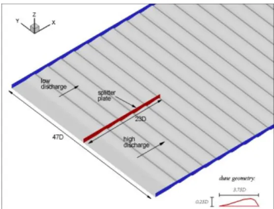
The Reynolds number defined with the channel depth, D (=0.067mm), and the mean velocity of the two currents, U0 (=0.23 m/s), is close to 15,500. The splitter length is 23D. The width of the channel is 47D and the length of the channel downstream of the splitter is 157D (=10.55 m) (Fig. 1). The channel bottom is smooth. The depth-averaged mean velocities of the two streams are U10=0.61U0 and U20=1.39U0, respectively. The mean velocities in the z/D=0.9 plane are 0.7U0 and 1.56U0, respectively. These conditions are similar to those present in the second test case studied by Uijttewaal and Booij (2000) where the streamwise velocity values at z/D~0.9 were used to estimate U10 and U20. The bed-friction velocities non-dimensionalized by the bulk velocity in each stream (U10=0.61U0 and U20=1.39U0, respectively) are 0.052 and 0.048. The spatial development of the shallow mixing layer is analyzed using DES on a mesh containing close to 10 million cells (912*336*32 in the streamwise, spanwise and vertical directions). The viscous sub-layer is resolved in the simulation and no-wall functions are used. In a second simulation, an array of identical 2D dunes is present. The wavelength of the dunes is 3.75D and their height is 0.25D. The dunes have a generic shape that approximates dunes developing in medium-size rivers. The equivalent non-dimensional bed roughness is close to 500 wall units (fully-rough regime).
The incoming flow contains realistic turbulence fluctuations obtained from two preliminary simulations with periodic boundary conditions in the streamwise direction. The free surface is treated as a rigid lid which is justified as the channel Froude number (Fr=0.28) is much less than one. The wall surfaces are treated as no-slip boundaries. Mass exchange processes are studied by considering the transport of a passive scalar for which an advection-diffusion equation is solved. The passive scalar is introduced continuously at the end of the splitter plate over the whole depth of the channel. The Schmidt number is assumed equal to unity. should be centred and should be numbered with the number on the right-hand side.
3. Results
Comparison of the instantaneous concentration fields from flatbed case in horizontal planes situated near the bed (z/D=0.1) and the free surface (z/D=0.9) in Fig. 2 shows the coherence of the quasi-2D eddies is decreasing as the channel bottom is approached. Also, there is a clear loss of the coherence of the large-scale eddies for x> 100D (~6.7 m, x is measured from the end of the splitter plate). This explains the observed decrease in the rate of growth of the mixing layer width in the streamwise direction (see discussion of Fig. 3) at all flow depths. The decay in the rate of growth increases with the decrease of the distance from the bed (see Kirkil and Constantinescu, 2008 for more details). The concentration contours in Fig. 2 suggest a rate of growth close to zero at z/D=0.1 for x/D>120D. Close to the free surface the average size of the largest eddies in the transverse direction is around 10D-15D (0.67-1.00 m) in the downstream part of the channel (x/D>120).
Comparison of the mean concentration profiles at z/D=0.9 and z/D=0.1 in Fig. 2 shows the positions of the centerline inferred from the mean streamwise velocity profiles and from the mean concentration fields are not identical. Based on the distribution of the mean concentration, the vertical tilt of centerline surface in the transverse direction is larger than 1.5D (~0.1 m) for x>120D. The vertical shift is slightly smaller in the case in which the velocity profiles are used to calculate the position of the centerline.
The development of the mixing-layer in the vertical direction is strongly non-uniform. This can be inferred from Fig. 2 where the width of the mixing layer inferred from the mean concentration field at a given streamwise location is significantly smaller at z/D=0.1 compared to z/D=0.9. Figure 3 allows a more quantitative comparison of the width of the mixing layer at different levels (z/D=0.1 and z/D=0.9) and in the depth-averaged flow. The width of the mixing layer in Fig. 3 was estimated based on the mean streamwise velocity
field. The local width of the mixing layer is defined as the maximum slope thickness (Uijttewaal and Booij, 2000):
𝛿𝛿 = 𝑈𝑈1−𝑈𝑈2
(𝜕𝜕𝜕𝜕/𝜕𝜕𝜕𝜕)𝑚𝑚𝑚𝑚𝑚𝑚 (1) where U1(x) and U2(x) are the streamwise velocities in the two streams at a given streamwise location, y is the spanwise direction and u is the streamwise velocity. The curves in Figure 3 are obtained by using eqn. (1).
Fig. 2. Contours of scalar concentration in the instantaneous (left) and mean (right) flow. a) z/D=0.9; b) z/D=0.1. The dashed-dot-dot line corresponds to the jet centerline determined from the mean concentration profiles. The dashed line corresponds to the jet centerline determined from the mean streamwise velocity profiles.
The results at z/D=0.9 are compared in Fig. 3 with two sets of measurements conducted at the free surface (van Prooijen and Uijttewaal, 2002) and 1 cm below the free surface (Uijttewaal and Booij, 2000). Up to x=2 m (30D) the mixing layer width at z/D=0.9 predicted by DES is close to the widths inferred from the two sets of measurements. Farther downstream, DES overpredicts the width compared to the experimental values. For example, at x=6 m (91D) DES predicts a width of 0.44 m, van Prooijen and Uijttewaal (2002) estimated a width of 0.38 m (the model equation used by the same authors to fit a smooth curve through their data predicted a value of 0.4 m), and Uijttewaal and Booij (2000) estimated a width of 0.32 m. At x=10.25 m (155D), DES predicts a width of 0.6 m. This is quite close to the value of 0.59 m estimated by van Prooijen and Uijttewaal (2002). The width (0.45 m) estimated by Uijttewaal and Booij (2000) is significantly lower. It is not entirely clear what is the reason for the relatively significant differences between the widths estimated from the two experiments, but DES predictions of the streamwise variation of the mixing layer width are clearly closer to the data of van Prooijen and Uijttewaal (2002).
Furthermore, the DES mean streamwise velocity fields are used to infer the streamwise variation of the mixing layer width close to the bed (z/D=0.1) and the streamwise variation of the width of the depth-averaged mixing layer. Such quantitative information on the vertical variation of the mixing layer width is not available from previous experiments. The differences with the values measured at or close to the free surface are significant for x>0.5 m (8D). For example, at x=2 m (30D) the mixing layer widths at z/D=0.9 and 0.1 are 0.185 m and 0.12 m, respectively, while the depth-averaged width is close to 0.16 m. At x=3.7 m, the depth averaged width (0.27 m) is roughly the mean of the values at z/D=0.1 (0.23 m) and z/D=0.9 (0.31). For x>4 m, the depth-averaged value is closer to the width measured close to the bed. This is because the width decreases relatively fast with the distance from the free surface in the upper layer of the channel and then much more gradually in the lower layer. For example, at x=10.25 m (155D) the width at z/D=0.1 (0.38 m) is about 30% lower than the width at z/D=0.9 (0.61 m). The width of the depth-averaged mixing layer is 0.47 m. The
field. The local width of the mixing layer is defined as the maximum slope thickness (Uijttewaal and Booij, 2000):
𝛿𝛿 = 𝑈𝑈1−𝑈𝑈2
(𝜕𝜕𝜕𝜕/𝜕𝜕𝜕𝜕)𝑚𝑚𝑚𝑚𝑚𝑚 (1)
where U1(x) and U2(x) are the streamwise velocities in the two streams at a given
streamwise location, y is the spanwise direction and u is the streamwise velocity. The curves in Figure 3 are obtained by using eqn. (1).
Fig. 2. Contours of scalar concentration in the instantaneous (left) and mean (right) flow. a) z/D=0.9; b) z/D=0.1. The dashed-dot-dot line corresponds to the jet centerline determined from the mean concentration profiles. The dashed line corresponds to the jet centerline determined from the mean streamwise velocity profiles.
The results at z/D=0.9 are compared in Fig. 3 with two sets of measurements conducted at the free surface (van Prooijen and Uijttewaal, 2002) and 1 cm below the free surface (Uijttewaal and Booij, 2000). Up to x=2 m (30D) the mixing layer width at z/D=0.9 predicted by DES is close to the widths inferred from the two sets of measurements. Farther downstream, DES overpredicts the width compared to the experimental values. For example, at x=6 m (91D) DES predicts a width of 0.44 m, van Prooijen and Uijttewaal (2002) estimated a width of 0.38 m (the model equation used by the same authors to fit a smooth curve through their data predicted a value of 0.4 m), and Uijttewaal and Booij (2000) estimated a width of 0.32 m. At x=10.25 m (155D), DES predicts a width of 0.6 m. This is quite close to the value of 0.59 m estimated by van Prooijen and Uijttewaal (2002). The width (0.45 m) estimated by Uijttewaal and Booij (2000) is significantly lower. It is not entirely clear what is the reason for the relatively significant differences between the widths estimated from the two experiments, but DES predictions of the streamwise variation of the mixing layer width are clearly closer to the data of van Prooijen and Uijttewaal (2002).
Furthermore, the DES mean streamwise velocity fields are used to infer the streamwise variation of the mixing layer width close to the bed (z/D=0.1) and the streamwise variation of the width of the depth-averaged mixing layer. Such quantitative information on the vertical variation of the mixing layer width is not available from previous experiments. The differences with the values measured at or close to the free surface are significant for x>0.5 m (8D). For example, at x=2 m (30D) the mixing layer widths at z/D=0.9 and 0.1 are 0.185 m and 0.12 m, respectively, while the depth-averaged width is close to 0.16 m. At x=3.7 m, the depth averaged width (0.27 m) is roughly the mean of the values at z/D=0.1 (0.23 m) and z/D=0.9 (0.31). For x>4 m, the depth-averaged value is closer to the width measured close to the bed. This is because the width decreases relatively fast with the distance from the free surface in the upper layer of the channel and then much more gradually in the lower layer. For example, at x=10.25 m (155D) the width at z/D=0.1 (0.38 m) is about 30% lower than the width at z/D=0.9 (0.61 m). The width of the depth-averaged mixing layer is 0.47 m. The
relative width reduction between z/D=0.9 and z/D=0.1 based on the velocity fields is consistent with the one estimated based on the mean concentration fields (e.g., see Fig. 3).
Fig. 3. Mixing layer width vs. downstream distance from the splitter obtained from the profiles of the mean streamwise velocity. Also shown are two sets of experimental measurements performed close to the free surface.
Finally, results from the simulation containing large-scale roughness elements in the form of an array of 2D dunes are discussed. The presence of the dunes increases significantly the total bed friction with most of the increase being due to the form or pressure drag component. Figure 4 shows the instantaneous concentration contours at the free surface along with the centerline inferred from the mean concentration contours. Several differences between the instantaneous concentration distributions in the z/D=0.9 plane in Figs. 2a and Fig.4 are observed. The concentration levels are lower in the case containing dunes. This is due to the scalar that is trapped in the recirculation region past the crest of the dunes and that diffuses in the spanwise direction, predominantly toward the lower speed side of the mixing layer. More importantly, the larger equivalent bed roughness induces a faster decrease of the entrainment coefficient which translates into a faster and larger shift of the mixing layer centerline (Fig. 5). For example, in the x=58D section, s/D=2.24 in the flat bed case and s/D=3.35 in the case with dunes. These values were obtained based on the mean concentration profiles. The values in the x=148D section are 4.79D and 7.16D, respectively. In fact, preliminary results suggest the equivalent bed roughness is high enough such that the growth rate of the mixing layer, in terms of its width and centerline shift, is almost zero for x/D>130 in the case containing dunes (Fig. 4).
4. Conclusions
DES predictions of the shallow mixing layer development close to the free surface were found to agree reasonably well with experimental observations. Meanwhile, the numerical results showed that the vertical variations of the width and centerline position of the shallow mixing layer are significant. For example, at distances between 75D and 150D from the splitter plate, the width of the mixing layer close to the free surface is 20-30% more than the width in the near-bed region.
The length of the domain was not sufficient for the mixing layer to reach the zero-growth regime in which the bottom friction effects become so large that the large-scale horizontal eddies cannot be sustained by the lateral shear and their coherence is gradually
lost. When bed roughness is increased due to the presence of 2D dunes, mixing layer reaches zero-growth regime faster.
Fig. 4. Instantaneous contours of scalar concentration for deformed bed case in a horizontal plane situated at 0.9D from the free surface.
Fig. 5. Variation of lateral shift of jet centreline with streamwise distance based on the analysis of flow fields at z/D=0.9
References
1. K.S. Chang, S. G. Constantinescu and S. Park “Assessment of predictive capabilities of
Detached Eddy Simulation to simulate flow and mass transport past open cavities,”
ASME J. of Fluids Engineering, Vol. 129(11), 1372-1383 (2007).
2. V.H. Chu and S. Babarutsi « Confinement and bed friction effects in shallow turbulent
mixing layers. » J. Hydraulic Engineering, Vol. 114, 1257:1274 (1988).
3. G. Constantinescu and K. Squires “Numerical investigations of flow over a sphere in the