ISTANBUL BILGI UNIVERSITY INSTITUTE OF GRADUATE PROGRAMS
FINANCIAL ECONOMICS MASTER’S DEGREE PROGRAM
DISTANCE TO DEFAULT FOR TURKISH BANKING SECTOR
SERCAN KOYUNLU 115624011
Dr. Öğr. Üyesi SEMA BAYRAKTAR TÜR
ISTANBUL 2019
PREFACE
This study is submitted in fulfilment of the requirements of the Master’s Degree of Financial Economics program at İstanbul Bilgi University. Banking has been so important today, especially for emerging countries like Turkey that depends heavily on the sector to fund the economy. In this context, the measurement and tracking of the riskiness of the banking sector are vital.
The study aims to measure the riskiness of the banking sector via distance to default concept, and it is questioned the distance to default is an early warning indicator for banking failure and crisis.
I would like to express my gratitude and thanks to my adviser Assistant Professor Sema Bayraktar Tür and my sister Ayşegül for her encouragement and help during my study.
Sercan KOYUNLU Istanbul,May 2019
TABLE OF CONTENTS
PREFACE iii
TABLE OF CONTENTS iv
LIST OF ABBREVATIONS vii
LIST OF SYMBOLS x
LIST OF FIGURES xii
LIST OF TABLES xiv
ABSTRACT xv
ÖZET xvi
INTRODUCTION 1
1 LITERATURE REVIEW 4
1.1 STUDIES ON BANK FAILURE . . . 4
1.1.1 Statistical-Based Models . . . 4
1.1.2 Artificial Intelligence Models . . . 8
1.1.3 Market-Based Models . . . 9
1.2 STUDIES ON BANK FAILURES IN TURKEY . . . 12
1.2.1 Statistical-Based Studies . . . 12
1.2.2 Artificial Intelligence-Based Models . . . 14
2 METHODOLOGY 19
2.1 THE CONCEPT OF OPTION . . . 19
2.1.1 What is the Option? . . . 19
2.1.1.1 Put Option . . . 19
2.1.1.2 Call Option . . . 21
2.2 THE MODEL . . . 22
2.2.1 Assumptions of the Merton Model . . . 22
2.2.2 Logic Behind Merton Model . . . 23
2.2.3 The Calculation of Probability of Default . . . 29
2.2.4 Determinants of Default . . . 30
2.2.5 Concept of Distance to Default . . . 31
2.2.6 Advantages of the Model . . . 32
2.2.7 Limitations of the Model . . . 33
3 DATA 34 3.1 Parameters of the Model . . . 34
3.1.1 Market Cap . . . 34
3.1.2 Liability and Default Barrier . . . 34
3.1.3 Risk-Free Rate . . . 35
3.1.4 Maturity . . . 35
3.1.5 Drift Rate . . . 35
3.2 Structure of the Data . . . 35
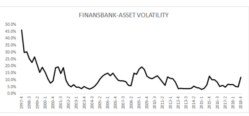
3.2.1 Steps to Follow . . . 36 4 EMPIRICAL RESULTS 42 4.1 Specific Results . . . 42 4.1.1 Non-failed Banks . . . 42 4.1.1.1 Akbank . . . 42 4.1.1.2 Albaraka . . . 43 4.1.1.3 Denizbank . . . 45 4.1.1.4 Finansbank . . . 46
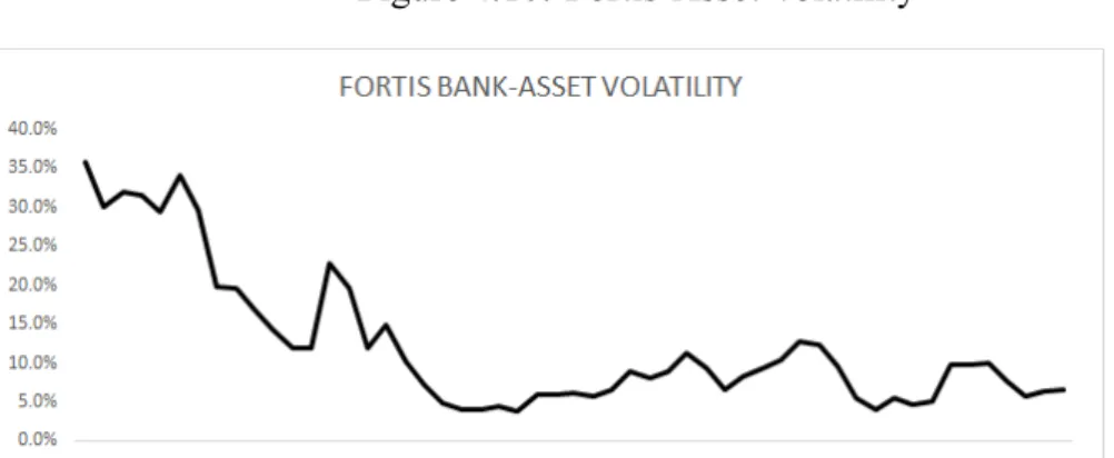
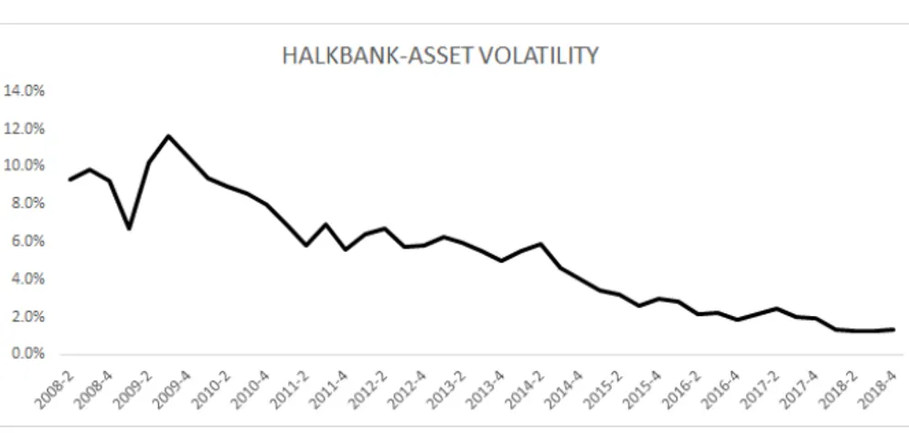
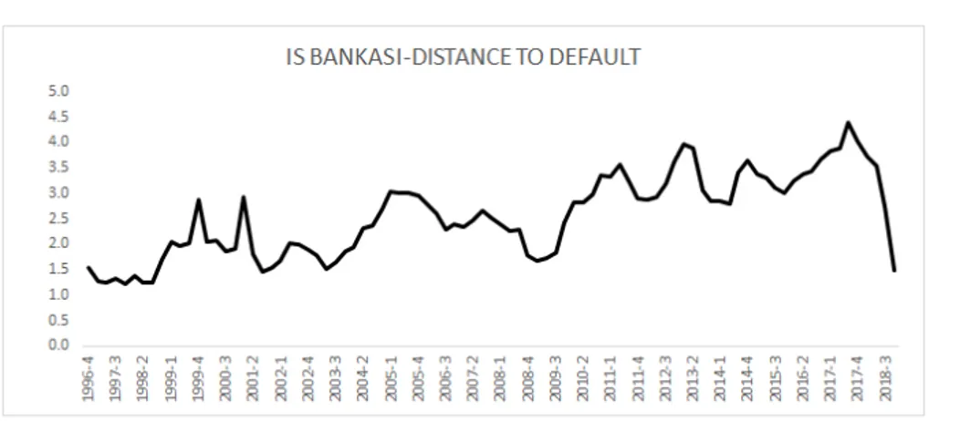
4.1.1.5 Fortis . . . 47 4.1.1.6 Garanti . . . 48 4.1.1.7 Halkbank . . . 49 4.1.1.8 Isbank . . . 50 4.1.1.9 TEB . . . 51 4.1.1.10 Vakifbank . . . 52 4.1.1.11 Yapi Kredi . . . 53 4.1.1.12 TSKB . . . 54 4.1.2 Failed Banks . . . 55 4.1.2.1 Asya Katilim . . . 56 4.1.2.2 Demirbank . . . 56 4.1.2.3 Toprakbank . . . 57 4.1.2.4 Tutunbank . . . 58
4.2 General Results for Turkish Banking Sector . . . 59
4.3 Forecasting Power of The Distance to Default . . . 61
4.3.1 Statistical Test of Indicators . . . 62
4.3.2 In Sample Forecasting . . . 64
CONCLUSIONS AND SUGGESTIONS 69
REFERENCES 70
LIST OF ABBREVATIONS
DD Distance to Default
BIST Borsa Istanbul
IEWS Integrated Early Warning System
PCA Principal Component Analysis
CAMELS Capital Adequacy, Asset Quality, Management, Earning Analysis, Liquidity, Sensitivity
KMV Kealhofer-McQuown-Vasicek
SDIF Savings Deposit Insurance Fund
TMSF Turkish Savings Deposit Insurance Fund
ANOVA Analysis of Variance
MLP Multilayer Perceptron
CL Competitive Learning
SOM Self-organizing Map
LVQ Learning Vector Quantization
ANN Artificial Neural Network
MDA Multivariate Discriminant Analysis
IMKB Istanbul Menkul Kiymetler Borsasi
PD/DD Market Value/Book Value
FDIC Federal Deposit Insurance Corporation
GDP Gross Domestic Product
SDIF Turkish Savings Deposit Insurance Fund
k-NN k-Nearest Neighbors
US United States
ID3 Iterative Dichotomiser
LIST OF SYMBOLS
σ Volatility
σA Asset Volatility
X Debt of a firm
ST Spot price of an option at maturity
S Spot Price
K Strike price of an option
p Put premium c Call premium P A Put payoff C A Call payoff rf Risk-free rate T Maturity
N() Cumulative normal distribution
W Wiener process
VA Asset value
µ Instantenous Drift
W Wiener process
VL Liability Value
LIST OF FIGURES
Figure 2.1: Short Put Payoff . . . 20
Figure 2.2: Long Put Payoff . . . 20
Figure 2.3: Short Call Payoff . . . 21
Figure 2.4: Short Call Payoff . . . 21
Figure 2.5: Default Process . . . 24
Figure 2.6: The value of equity at maturity . . . 26
Figure 2.7: The relationship between firm asset value and liabilities at maturity . . . 27
Figure 4.1: Akbank-Distance to Default . . . 43
Figure 4.2: Akbank-Asset Volatility . . . 43
Figure 4.3: Albaraka-Distance to Default . . . 44
Figure 4.4: Albaraka-Asset Volatility . . . 45
Figure 4.5: Denizbank-Distance to Default . . . 46
Figure 4.6: Denizbank-Asset Volatility . . . 46
Figure 4.7: Finansbank-Distance to Default . . . 47
Figure 4.8: Finansbank-Asset Volatility . . . 47
Figure 4.9: Fortis-Distance to Default . . . 48
Figure 4.10: Fortis-Asset Volatility . . . 48
Figure 4.11: Garanti Bankasi-Distance to Default . . . 49
Figure 4.12: Garanti Bankasi-Asset Volatility . . . 49
Figure 4.13: Halkbank-Distance to Default . . . 50
Figure 4.14: Halkbank-Asset Volatlity . . . 50
Figure 4.16: Isbank-Asset Volatility . . . 51
Figure 4.17: TEB-Distance to Default . . . 52
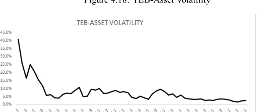
Figure 4.18: TEB-Asset Volatility . . . 52
Figure 4.19: Vakifbank-Distance to Default . . . 53
Figure 4.20: Vakifbank-Asset Volatility . . . 53
Figure 4.21: Yapı Kredi-Distance to Default . . . 54
Figure 4.22: Yapı Kredi-Asset Volatility . . . 54
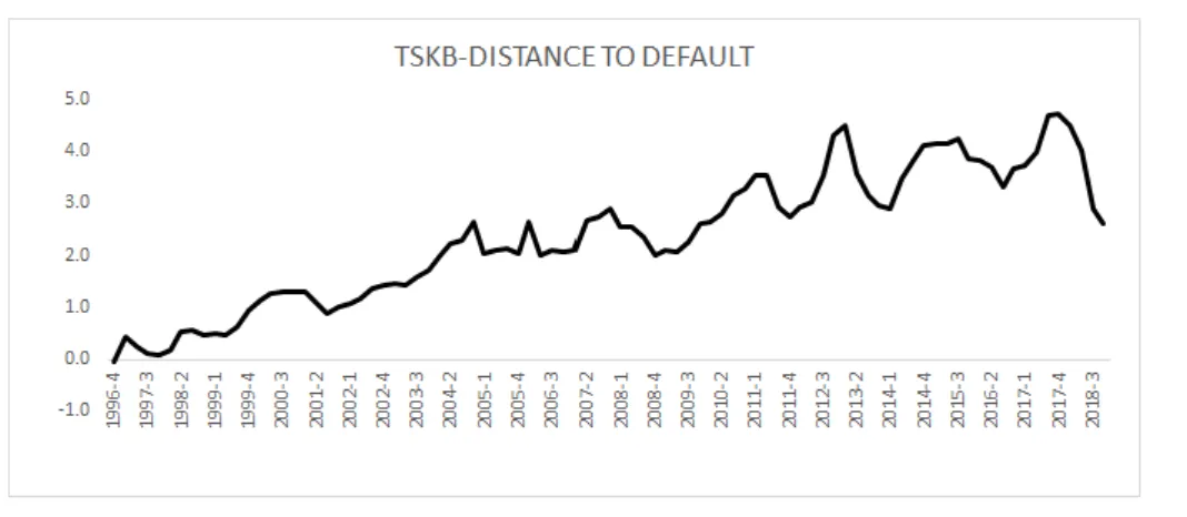
Figure 4.23: TSKB-Distance to Default . . . 55
Figure 4.24: TSKB-Asset Volatility . . . 55
Figure 4.25: Asya Katılım-Distance to Default . . . 56
Figure 4.26: Asya Katılım-Asset Volatility . . . 56
Figure 4.27: Demirbank-Distance To Default . . . 57
Figure 4.28: Demirbank-Asset Volatility . . . 57
Figure 4.29: Toprakbank-Distance to Default . . . 58
Figure 4.30: Toprakbank-Asset Volatility . . . 58
Figure 4.31: Tutunbank-Distance to Default . . . 59
Figure 4.32: Tutunbank-Asset Volatility . . . 59
Figure 4.33: Turkish Banking Sector-Distance to Default . . . 60
LIST OF TABLES
Table 2.1: Payoff Structure . . . 28
Table 3.1: Banks used in this study . . . 36
Table 3.2: Sample Size . . . 37
Table 3.3: Cubic Spline Interpolation-YAPI KREDI-2018-Q4 . . . 41
Table 4.1: The Test Results of Difference of the Means Between Failed and Non-failed Banks . . . 62
Table 4.2: Summary of Welsch t-test Results-2001 Crisis . . . 64
Table 4.3: Summary of Welsch t-test Results-2008 Global Crisis . . . . 64
Table 4.4: Summary of Welsch t-test Results-2018 Currency Volatility Hike . . . 64
Table 4.5: Probit Regression Results . . . 66
Table 4.6: Logit Regression Results . . . 67
Table 4.7: LR Statistics of The Models . . . 67
Table A1: 2001 Crisis-Test Of Equality before 12 Months . . . 75
Table A2: 2001 Crisis-Test Of Equality before 9 Months . . . 75
Table A3: 2001 Crisis-Test Of Equality before 6 Months . . . 75
Table A4: 2001 Crisis-Test Of Equality before 3 Months . . . 76
Table A5: 2008 Global Crisis-Test Of Equality before Months . . . 76
Table A6: 2008 Global Crisis-Test Of Equality before 6 Months . . . . 76
Table A7: 2008 Global Crisis-Test Of Equality before 9 Months . . . . 76
Table A8: 2008 Global Crisis-Test Of Equality before 12 Months . . . . 77 Table A9: 2018 Currency Volatility Hike-Test Of Equality before 3 Months 77
Table A10: 2018 Currency Volatility Hike-Test Of Equality before 6 Months 77 Table A11: 2018 Currency Volatility Hike-Test Of Equality before 9 Months 77 Table A12: 2018 Currency Volatility Hike-Test Of Equality before 12
Months . . . 78 Table A13: Distance to Default-Turkish Banks-First Part . . . 78 Table A14: Distance to Default for Turkish Banks-Second Part . . . 81
ABSTRACT
This thesis examines the riskiness of the Turkish Banking system analyzing 16 banks traded at Borsa Istanbul(BIST) Banking Index between 1996 and 2018 by using a structural approach known as the Merton Model. Also, whether the model is a good predictor of the financial crisis and financial failure is investigated. Since the lit-erature is heavily dependent on accounting-based models and artificial intelligence models, the alternative measurement for riskiness for Turkish Banks is suggested. In this context, the distance to default based on Merton’s structural approach is mea-sured and via suitable logit and probit model is converted to the default probability. Using these results, whether the model can be used as an early warning indicator for the crisis and bank failure is examined. According to the results, the logit and probit model is statistically significant at 1% level of significance up to 12 months. The results also show that DD, in the case of Turkish Banking Sector, can be useful as an early warning indicator for banking failure but, there is no evidence that it can be helpful to detect economic crisis.
ÖZET
Bu tezde, 1996 ve 2018 yılları arasında BIST’te işlem görmüş 16 banka Merton Modeli olarak bilinen yapısal yaklaşım analiz edilerek Türk Bankacılık Sisteminin riskleri incelenmiştir. Ayrıca modelin finansal krizlerin ve finansal başarısızlıkların iyi bir tahmincisi olup olmadığı araştırılmıştır. Literatür, ağırlıklı olarak muhase-beye ve yapay zeka modellerine dayalı olduğundan, Türk Bankaları için alternatif risklilik ölçüm yöntemi önerilmiştir. Bu kapsamda Merton’un yapısal yaklaşımı kul-lanılarak, temerrüde olan uzaklık ölçülmeye çalışılmış ve probit ve logit regresyon aracılığıyla temerrüde olan uzaklık temerrüt olasılığına dönülmüştür. Bu sonuçlara göre temerrüde olan uzaklık ölçüsünün krizleri ve banka başarısızlıklarını açıkla-mada erken uyarı göstergesi olarak kullanılıp kullanılmayacağı analiz edilmiştir. Bulgulara göre, logit ve probit regresyonlar 12 aya kadar 1% önem düzeyinde is-tatistiksel olarak anlamlı çıkmıştır. Ayrıca sonuçlar, temerrüde olan uzaklığın fi-nansal başarısızlıkları tahmin etmede anlamlı olduğunu krizlerin tahmin edilmesi için erken uyarı göstergesi olarak kullanılmasına yönelik yeterince kanıt olmadığını göstermiştir.
INTRODUCTION
The detection of the soundness of a banking sector is so crucial because when the banking system enters a crisis or failure state, then the credit channel does not func-tion very well and an economy is entirely affected especially in the countries that are highly dependent on the banking system and where the capital market system is undeveloped. Furthermore, in the case of banking failures, society pays a substan-tial cost, and it affects all segments of society, especially taxpayers. According to the financial services sector report1, the banking system captures 67% of the total assets of the financial sector in Turkey. Since financial markets are not developed in Turkey, the banking system is quite important for companies to reach financing. For these reasons, I implement the model suggested by Merton (1974) to Turkish Banks to monitor the riskiness of the banking traded at BIST for the period between 1996 to 2018.
Option-based or structural models have already been widely used to measure the credit risk of non-financial firms. Merton’s " On the Pricing of corporate debt " study published in 1974 led to many academic studies implementing this model to many various areas. One of them is the KMV, successful commercial version of the Merton model.
The main objective of this study is to implement structural models in measuring the risk of banks in Turkey. The literature about banking failure in Turkey is excessively based on statistical methods and artificial intelligence methods such as support vec-tor machines, neural networks etc. and most of the studies compare statistical
meth-1
ods and artificial intelligent methods in the success of prediction ability. There are not enough number of studies using structural models in Turkey. This thesis will contribute to the literature by implementing Merton based model in measuring and tracking of the riskiness of the Turkish banking sector. Outputs of the model can be used to create an early warning system for the banking sector. As Rose and Ko-lari (1985) said that banking closure is not an immediate consequence. Most of the failed banks show some sign of the failure before closure.
According to Sinkey Jr (1975), one of the advantages of effective early warning sys-tems is that resources can be allocated more efficiently and the examination costs could be reduced.
In the academic environment, the model has been widely used for measuring the credit risk for non-financial firms and some authors also implemented for banks. However, it is debatable whether the model is sufficient or not. From supporting sides, Hillegeist et al. (2004) argue that the Merton model is superior to Altman’s discriminant analysis and Ohlson’s o-score based on logistic regression.
When it is compared to accounting-based bankruptcy prediction methods, there is no theoretical foundation for accounting-based models, contrary to option-based mod-els(Agarwal and Taffler, 2008). In other words, accounting-based models are sample specific. Besides, Agarwal and Taffler (2008) stress that accounting ratios in nature measure past performance, so it cannot be an indicator for the future performance and accounting records can be manipulative, and there is a possibility that the as-sets are not recorded with real value. According to Agarwal and Taffler (2008), Merton-based models provide a theoretical explanation for explaining the failure of companies. In efficient markets, market-based models can cover more information than accounting-based models, and the results of the model are independent of time and sample.
Also, according to Chan-Lau et al. (2004), market prices can tell us about bank con-ditions. According to them, the advantage of using market prices stems from the high frequency of the data, and they claim that the model is useful. As evidence, they claim that the model correctly forecasted the Argentian crisis in advance before
nine months.
The thesis will be divided into five parts. In the first part, the literature about studies related to banking failure in Turkey and the other essential studies except Turkey will be discussed. Methodology part covers a brief summary of the options and Merton-based approach. In the third part, the data will be analyzed. The following section will present empirical results, and in the last part, the conclusions drawn in light of the results will be discussed.
CHAPTER 1 LITERATURE REVIEW
1.1 STUDIES ON BANK FAILURE
The financial failure methodologies can be grouped into three types; statistical-based, artificial intelligence models and market-based models. In the types of statis-tical based models, the ultimate aim is to find the best variables that mostly discrim-inate between failed and non-failed firms. Typically, there is no robust framework in determining variables or equations and the variables that affect the default pro-cess are weighted. Some of them are discriminant analysis, logit regression, probit regression, multivariate discriminant analysis, and so on.
The second type is the artificial intelligence models. Contrary to statistical-based models, there are no statistical assumptions, and like statistical models, generally, they have no robust framework explaining the default process. Some of them are neural networks, fuzzy clustering, and so on.
The third type is market-based models, and they give a framework that explains the default process, contrary to other kinds of models and they are dynamic because they extract the default information from the share prices. In this context, the the other types can be classified as static models.
1.1.1 Statistical-Based Models
Sinkey Jr (1975) tries to estimate the bank failures with the help of balance sheet and income statement. The method of multivariate discriminant analysis is chosen.
The data consist of the banks identified as problematic at by FDIC. At 1972, there were 90 problematic banks, and at 1973, there were 20 failed banks. Each failed bank was matched according to specific criteria. His findings were that for between 1969-1971, efficiency, and other expenses were the most critical factors in discrim-inating the failed and the healthy banks, for 1972, loan volume and loan quality was the most important early warning signals.
Lane et al. (1986) is the first group of academician implementing Cox proportional hazard model to bank failure issue. They estimate two versions. One of them is the 1-year model that predicts the likelihood that survives from 0 to 12 month and the other one is the 2-year model that predicts the probability that survives from 12 to 24 month. The data sample consist of 130 failed and 334 non-failed banks from 1979 to 1983. They compare the Discriminant analysis with the Cox proportional hazard model. The results show that they performed equally well, but in terms of type I, the latter was more successful.
Pantalone et al. (1987) analyze the increase in bank failure in the US states during the 1980s. They try to investigate the cause of the surge in bank failure in decades. They claim that in essence, in overall bank management quality determines whether the bank will fail or not. Deregulation is not the leading causes of bank distress. They make use of the balance sheets and income statements to construct a logit model that forecast the commercial bank failure prior to one and two years. In building model, they have used five categories; profitability, management efficiency, lever-age, risk/diversification, and the state of the economy. The sample included 44 failed banks in 1983, and 69 failed banks in 1984 in sum 113 failed banks, and 226 healthy banks at random. They divide the sample data into four groups; 4.group is used as a test group. The model’s variables are net income/total assets, equity/total assets, loans/total assets, commercial loans/total loans and the absolute value of change in residential construction. The results are satisfactory. Prior to 1 year, the model esti-mates the failure correctly at 92%. Prior to 2 years, this rate is 89%. Also, Pantalone et al. (1987) stress that the economic downturn and the state of the economy is not the reason for bank failure; the real reason stems from the internal management
qual-ity.
Thomson et al. (1991) make a point about the large bank failures throughout the 1980s. However, the aim of the study is to construct the model estimating the fail-ure of banks including all sizes, not just large banks. Thomson et al. (1991) allege that the logit model can be used to determine the failure prior to 4 years. The data sample includes the year between 1984 and 1989, while the number of non-failed banks is 1736, the failed banks are 78, 78, 115, 133, 193, 175 in 1984, 1985, 1986, 1987, 1988, and 1989 respectively. They choose the logit model because the or-dinary least squares model has restrictive assumptions, and logit model is advanta-geous over probit since logit is not sensitive to the uneven sampling frequency issue. According to the findings, the model includes the variables related with capital ad-equacy, asset quality, management quality and earnings performance, liquidity and the economic state and all of them affect the failure prior to 4 years. The logit model has good classification results in sample and holdout samples. While the model clas-sifies correctly 93% up to 1 year, classification accuracy reduces to 82% prior to 4 years. Thomson et al. (1991) conclude that the logit model could be used as an early warning system.
Whalen et al. (1991) analyze the failed US banks between 1987 and 1991 with the help of the Cox proportional hazard model. This type of model produces the proba-bility that the bank will survive at a specific period. Also, this study is, to some ex-tent, is different in sampling selection. They criticize the matched sample selection since it is based on the subjective assessment. The sample data include randomly selected roughly 1500 non-failed banks and failed banks at the relevant period. The estimation sample consists of the failed banks in 1987 and 1988 and approximately 1000 non-failed banks. The remainder is used to as a hold-out sample. The model es-timates the probabilities that the bank will survive longer than 0 years to 24 months. For explanatory variables, the end of 1986 data are used, and the financial ratios are obtained from the call reports and local economic state indicator, the percentage change in state residential housing permits issued are added to the model. According to the model results, the ratios that affect the probability of bank survival was
over-head expense ratio, the large certificate to deposit ratio, the loan to asset ratio, the primary capital ratio, the nonperforming loan ratio, the net primary capital ratio and local indicator related with housing. Results show that the Cox proportional hazard model can be used as an early warning system since low type I and type II errors are small and classification accuracy was high at 12-, 18-, 24- month prediction. Cole and Gunther (1998) try to construct a bank failure estimate based on probit model. They argue that the efficiency and the information content of CAMEL’s rat-ing built based on on-site examination are fairly decayrat-ing as time passes. Therefore, it must be complemented by the off-site examination, namely early warning systems. CAMEL ratings do not respond to changing financial conditions very well. So they formed an early warning model based on probit model. Their model uses the end of 1985 and 1987 financial ratios and 13966 US commercial banks. One of the models uses 1985 ratios; the other model uses 1987 financial ratios. For two models, the variables that explain the failure was equity, past due loans, nonaccrual loans, other real estate owned, net income, investment securities and large certificate of deposits and they are found to be statistically significant at 1% level.
Demirguc-Kunt and Detragiache (2005) update the model introduced by themselves at 1998 paper. Their approach is the multivariate logit approach. But their approach is much more related to a systemic banking crisis, not specific bank failure mea-surement. So their dependent variable is the crisis. If the banking crisis happens, then the dependent variable is equal to 1, otherwise to 0. The model measures the fragility of the banking system. They extend their work of 1998 by enlarging the sample to 94 countries and extending the sample period to 2002. The number of a banking crisis at this period increased from 31 to 77. They conclude that the banking crisis is highly interconnected with high inflation, high real interest rates and low GDP growth.
Kolari et al. (2002) examine the large bank failures, and they compare the paramet-ric approach and the non-parametparamet-ric approach to create an early warning system. They choose the logit analysis as the parametric and trait recognition as the non-parametric approach. As a sample, they use the failed 50 large banks with asset
size greater than 250 million USD throughout the 1980s. The data group includes two groups as the original sample and hold-out sample. To create an original sam-ple, they choose 25 failed banks and 25 healthy banks. In terms of classification results, both of them show equal success; however, at hold-out samples, trait recog-nition pattern showed much better performance in terms of overall accuracy and large bank failure accuracy. The expectation is that trait recognition performs better at small samples. Their results verify this idea, and they claim that trait recognition patterns catch 2- and 3-variable interaction between variables about the failure risk. According to these results, trait recognition pattern estimates large bank failures highly accurately prior to 1 and 2 years.
1.1.2 Artificial Intelligence Models
Tam and Kiang (1992) have one of the first studies that used artificial intelligence(AI) models in the subject of bank failure. They compare neural networks and discrim-inant analysis techniques. Their sample includes the banks at Texas banks failed between 1985-1987. They use 59 failed and 59 non-failed banks as training data. They compare the neural network approach to logistic regression, k-NN, and ID3 by using bankruptcy data of the banks. According to results, the neural-net approach offers an alternative to existing bankruptcy prediction models.
Alam et al. (2000) implement fuzzy clustering algorithms and self-organizing neu-ral networks to predict the potentially failed banks. They compare two models, and criticize the general dichotomous models whose inputs are failed and nonfailed only try to separate the banks as failed and healthy. They stress the importance of a rel-ative degree, and they argue that the fuzzy clustering algorithms assess the banks on a continuous scale, not a dichotomous scale. They also criticize the studies that include equal sample failed and non-failed banks. They choose 24 US banks re-ported at FDIC Annual Report as failed at 1992. They eliminate 14 banks at random and after they eliminate two banks also because of lack of data and they matched each failed bank with 30 healthy banks. They divide the sample into 3 groups and 9 clusters. They implement fuzzy clustering and self-organizing neural networks.
According to the findings, fuzzy clustering and self-organizing neural networks are satisfactory to determine potentially failed banks.
Salchenberger et al. (1992) compare the logit model and neural network approach for the estimation of failure of thrift(Savings and Loans Association) failures. The data set includes 34.795 savings and loans institutions for the period of January 1986 to December 1987. June 1986’s call reports are used as a training set. Three sample sets are used to test the models. At the first sample, 100 failures are matched with 100 non-failed savings and loans associations according to the geography and asset size. The second sample is used to test the predictive abilities of the two models. For each failed institution, the data was compiled 6, 12 and 18 months prior to fail-ure. For 12 months, 58 failed banks’ data are found; for 18 months, 24 failed banks’ data are found. A third sample was called as “diluted sample”. The diluted sample is constructed and 75 failures matched with 329 non-failed institutions. The two cutoff points are determined. They are 0.2 and 0.5 for both models. And they find that the decrease in cutoff point has a much more significant impact on logit results related to classification issue. In other words, when the cutoff point reduces, then type II errors increase more for the logit model. They also allege that at all samples, the neural network approach was at least sound as the logit approach; in some cases, it performs better.
1.1.3 Market-Based Models
The third popular method for analyzing the riskiness of firms is market-based mod-els. These models evaluate the riskiness by looking at the changes in the market value of firms.One of the important studies using this method is the one by Chan-Lau et al. (2004). They try to construct a bank vulnerability indicator for emerging countries through the distance to default based on Merton structural model. The data sample includes 38 banks from developing countries. According to the results, the model can predict bank trouble in advance up to nine amounts. They say that the distance to default can be beneficial in supervising banks. The sample is between 1997 and 2003. They argue that in times of East Asian Crisis, distance to default
has reached its peak level and banks’ shares reacted to this event, and their volatility increased, and asset value decreased so that the model can explain the fundamentals of the banks. To test econometrically, due to lack of sufficient distressed bank, they define credit event as the decrease in the rating to CCC assigned by Moody’s, Fitch or Standard and Poors. For 3-, 6-, and 9- month forecasting horizon, absolute value DD for downgraded banks is lower than non-downgraded banks according to Welch t-test. Then to test in-sample forecasting power for 3-,9- and 12-month forecasting horizon, Chan-Lau et al. (2004) use probit and logit regression where PD is depen-dent and DD is the independepen-dent variable. And they conclude that at 5% significance level prior to 9 months, DD is a crucial tool for early warning. To test out-of-sample, 2 Argentian Banks are chosen that are downgraded at the near of Argentinian crisis in 2001.
Another study by Bichsel and Blum (2004) investigates the relationship between leverage ratio and capital and the relationship between the probability of default and the capital ratio. Their sample includes 19 Swiss commercial banks between 1990 and 2002.The study use z-scoreas the probability of financial failure. The re-lationships are analyzed with the panel regression analysis. According to the results, as more capital encourages to taking more risk, and there is no significant relation-ship between default and capital ratio.
Gropp et al. (2006) are another group of academicians that argue that DD and bond spreads can give a signal before the failure. They analyzed European Banks operated between 1991 and 2002. Since there are no failed banks if FITCH rating is below C, then the banks are flagged as fragile, and they compare and test the predictive power of bond spreads and DD. According to the results, the bond spread is very respon-sive near default, but it does not give a signal for periods longer than six months. However, DD gives a signal up to 24 months. Also, they analyzed whether DD is unbiased and complete. They conclude that DD is complete because it includes all factors determining default such as asset risk, leverage and earnings expectations and also is biased because it measures the default correctly.
MDA. Lane et al. (1986) also used discriminant analysis to analyze bank failures and compares with the Cox proportional hazard model and the latter is found to be more successful. Whalen et al. (1991) estimated the financial crash up to 24 months with the Cox proportional hazard model. The logit model was used by Thomson et al. (1991), Pantalone et al. (1987), Kolari et al. (2002), and Demirguc-Kunt and De-tragiache (2005). Demirguc-Kunt and DeDe-tragiache (2005) construct the model on a banking sector, rather than bank level. Also, Kolari et al. (2002) use trait recog-nition, and in terms of failure accuracy, it is more successful than the logit model. Cole and Gunther (1998) used the probit model to explain bank failure. Tam and Kiang are one of the academicians comparing the neural network and discriminant techniques in terms of bank failure. Alam et al. (2000) use fuzzy-clustering algo-rithms and self-organizing maps. They criticize dichotomous perspective so suggest fuzzy-clustering based on a dichotomous scale. Salchenberger et al. (1992) assert that the neural networks are at least as good as logit models in some cases, they are more successful. Chan-Lau et al. (2004) implemented structural models to bank failure, and they allege that DD is a good indicator for bank failure up to 9 months.
1.2 STUDIES ON BANK FAILURES IN TURKEY
1.2.1 Statistical-Based Studies
Canbas et al. (2005) analyze 40 Turkish private banks between 1997 and 2003 and the sample includes 21 failed banks. They aim to create an "integrated early warn-ing system(IEWS)” to detect financial problems early. They use probit analysis, logit analysis and discriminant analysis to create IEWS. The reasons that change the bank profile have been searched by the method of principal component analy-sis(PCA). They claim that the most critical characteristics that change the bank’s health are capital, income-expenditure structure and liquidity. They also find that PCA is more useful to account for the features of the Turkish banking sector than CAMELS.
Doğanay et al. (2006) analyze the banks operating in Turkey between 1997 and 2002. Doğanay et al. (2006) use the probit model, the logit model and the discrimi-nant analysis like Canbas et al. (2005) did, to detect financial failure prior to 3 years by using financial ratios. The results of the study show that the best model explain-ing Turkish Bank failure is the logit model.
Çinko et al. (2008) use the CAMELS rating system for the Turkish banking sector between 1996 and 2001 and conclude that CAMELS rating is not applicable for the Turkish Banking system. According to this study, banks that are captured by SDIF have higher CAMELS rating than banks that are not captured. This study analyzes whether the discriminant analysis, logit analysis and artificial neural networks can accurately predict which banks will be seized by SDIF with the help of CAMELS rating ratios. All the models produce the same result, but the models are not satis-factory in predicting which banks will be seized by SDIF.
Erdogan (2008) tries to create a logistic model that estimates the financial failure for the Turkish banking sector. Data period is between 1997-1999. The estimated period is 1999-2001. He argues that the logit model produces good results in es-timating financial failure and financial failure could be estimated prior to 2 years. Erdogan (2008) argues that the logit model produces good results in estimating
fi-nancial failure. Erdogan advocates the logit model because the logit model does not require the normality assumption. Significant variables for this model are share-holder’s equity+total income/(deposits+non-deposit Funds), net income(loss) aver-age total assets, net income(loss)/ averaver-age share-in capital, interest income/interest expenses, non-interest income/non-interest expenses, and provision for loan losses/ total loans.
Ruzgar et al. (2008) examine the financial failure prediction model for 41 banks operating between 1995 and 2007. They use the rough set theory and 36 financial ratios. According to the paper, in Turkey, the most important parameter that sepa-rates the failed and healthy banks is the capital ratio, and the models that are based upon the statistical methods can be used as an early warning indicator.
Ünvan and Tatlidil (2011) analyze the effects of banking regulations and supervi-sions made after the 2001 crisis and question whether the financial ratios affect bank failure. In this context, 70 banks operated between 2000 and 2008 are analyzed, and 37 financial ratios are utilized in compliant with CAMEL ratios. Then Ünvan and Tatlidil (2011) compare logistic, probit and discriminant models. According to re-sults, discriminant analysis is the best method for bank failure prediction and, low income, liquidity, and the existence of risky assets play an essential role in bank failure.
Ilk et al. (2014) aim at modelling the financial failure in the Turkish banking sector with the help of principal component analysis. They analyze a sample including 40 banks operating between 1998 and 2000 by using three models; logistic regression, logistic regression that takes serial correlation into account via generalized estimat-ing equations, and a marginalized transition model. They find that each model clas-sifies the failure correctly at 93.3%. But statistically, marginalized transition model performs better than other models. They claim that their paper is unique because the panel data was never used in bank failure prediction studies before. They also claim that even though they use the same data sample with Canbas et al. (2005), they are more successful than their study because of the use of the panel data. Additionally, they criticize Canbas (2005) study in the method of selection of the variables
af-fecting financial failure. They assert that the use of ANOVA is not an appropriate solution to select variables because financial data does not distribute normally. For this reason, they claim principal component analysis is more suitable in the selection of variables.
Ozel and Tutkun (2014) try to fit the Cox regression model to predict bank failure for Turkish banks. Their studies are unique because there is no other study to use Cox regression model to estimate bank failure of Turkish banks. The data include all 70 Turkish Banks operated between 2000 and 2008. For analysis, they utilize 37 financial ratios. The additional important point is that Ozel and Tutkun (2014) ana-lyze all banks, not just commercial banks. According to their findings, no-stratified Cox regression model outperformed the logistic regression and other survival mod-els. Low income, liquidity, and the existence of risky assets play an essential role in a bank failure, as Ünvan and Tatlidil (2011) stress.
Erdogan (2016) uses panel data to create an early warning system for bank failure estimation. The sample is the commercial banks operated between 2000 and 2012. He stresses that there are a few studies using panel data to forecast bank failure. He analyzes panel data using pooled logistic regression and random logistic regression. The study is also different in terms of the definition of bank failure. Failed banks are determined according to the return on assets because of the limited data of failed banks. Return on asset is used as the dependent variable. Independent variables are found via factor analysis. These are interest income and expenditures, equity, other income and expenditures, deposit, due, asset quality. According to the findings, both methods can extract useful information for financial failure.
1.2.2 Artificial Intelligence-Based Models
Kilic (2006) applies electre-1 model based on multicriteria decision analysis for 40 Turkish Banks. The aim is to create an early warning system to detect the problems prior to 1 year. Kilic (2006) compares the electre-1 model to Canbas et al. (2005)‘s results. Kilic (2006) finds that electre-1 model has 93% classification success and makes a comparison in terms of type I error and type II error. According to results,
the probit model has the smallest type-I error, and Electre-1 model has the lowest type-II error.
Boyacioglu et al. (2009) implement support vector machines, artificial intelligent methods including and various statistical methods to predict financial failure in Turkish banks. Statistical methods used are k-means cluster, logistic regression and multivariate discriminant analysis. Twenty financial ratios were detected and grouped under 6 groups, based on CAMELS. The data sample includes 21 failed banks taken over by SDIF and 44 non-failed banks between 1997 and 2003. The data were divided into a training set including 14 failed and 29 non-failed banks and validation set including 7 failed and 15 non-failed banks. Then, financial ra-tios were tried to be eliminated. 12 variables were dropped based on t-test. After this procedure, Boyacioglu et al. (2009) find that the factor analysis is suitable via Kaiser-Meir-Olkin test and Bartlett’s test of sphericity and then implemented PCA and 7 factors are found to explain over 80% of the variance, so statistical meth-ods constructed have 7 variables. According to the results, Boyacioglu et al. (2009) show that at the validation set the MLP type of ANN is the most successful meth-ods, at training set, LVQ is the most successful method in terms of classification rate with over 90% classification rate and SVM and ANN types of models are superior to statistical methods in terms of classification rates.
Mazibas and Ban (2009) use neural networks to separate healthy and failed banks prior to default by using 36 financial ratios between 1995 and 2001. Their aim is to create an early warning system based on neural networks, and they compare the relative strength of neural network models with statistical methods such as probit and discriminant analysis in terms of failure prediction. They criticize that statisti-cal methods have many assumption limitations, and they do not capture non-linear structure in estimating financial failure. On the contrary, neural networks do not have any requirement to build a model. Hence, neural networks models have ad-vantages over statistical methods. Mazibas and Ban conclude that artificial neural networks are better than statistical methods in estimating financial failure.
and multivariate discriminant analysis in predicting financial distress. They find that neuro-fuzzy has 90.91%, ANN has 86.36%, and MDA has 81.82% of accuracy in classifying the banks. They find that neuro-fuzzy is much better than other models. Also, according to them, it is hard to interpret the coefficients of ANN, so how the model is created is not clear.
Ecer (2013) uses support vector machines and artificial intelligence models to pre-dict financial failure. According to Ecer (2013), as Mazibas and Ban (2009) stress, these type of models capture the nonlinear relationship better than statistical models. Data set chosen include 34 banks, 17 failed not the remaining not failed, operating between 1994 and 2001. 36 financial ratios are chosen, but with the help of ANOVA, Ecer (2013) eliminated 22 financial ratios. The aim is to make a comparison between these models. The conclusion is that two models are rather satisfactory, but the ar-tificial neural network is slightly better than support vector machines in predicting financial failure of banks in Turkey.
1.2.3 Market-Based Studies
Suadiye (2006) analyzes the banks traded at IMKB between 1997 March and 2006 March. The data sample consists of 12 banks but because of data suitability, 3 banks are dropped from the sample. The aim of the study is to measure the riskiness of Turkish commercial banks and predicting the relationship between capital level and risk level of banks. Merton option pricing methodology is used to predict default risk of Turkish commercial banks and is questioned whether there is a significant relationship between capital level and riskiness via panel data analysis. The results show that as the level of capital increases, banks take more risk, but their probability of default decreases because the market perceives an increase in capital positively. Sayılır (2010) implements logit models and Merton model to compare terms ana-lyzed. She divides the study into two parts. In the first part, banks operated between 1997 and 1998 are chosen, and then logit models are constructed. The first one takes only consideration accounting ratios, which are net profit/total assets, non-interest incomes/non-interest expenses, liquid asset/total assets, equity/total assets and total
loan/total assets. According to first logit model result, non-interest income/non-interest expense is a significant parameter at the 5% significance level and equity/-total asset at 10% significance level that separate banks taken over SDIF and banks not taken by SDIF. In the second logistic model, accounting ratios and market ratios, which are the difference between index return and share return, PD/DD, and the stan-dard deviation of daily return for 3 months are combined. In this model, in addition to previous variables, market value over book value is also statistically significant at 5%. In the second step, for 9 banks the structural model is implemented to measure the probability of default between 1997 and 2006. According to the conclusions, adding the market variable to the logit model increases the explanatory power of the model, and when compared to 1997 and 2006 by looking at PD and doing t-tests, the probability of default decreases structurally because of the measures taken after the 2001 crisis.
In this thesis, for the Turkish Banking sector, and banks at the sample, distance to default are calculated during 1996 and 2018. Thanks to long-range time, the consis-tency of DD will be tested. In recent literature, there is not enough study based on structural methods analyzing Turkish Banks, so I hope that from this angle, it will contribute the literature in the Turkish Banking sector. Also, by testing logit and probit models, the model suggesting the relationship between PD and DD will be created for the Turkish banking system. In nature, the DD model is forward-looking, contrary to other types of models. So, it is considered that updated DD numbers will shed light on the current riskiness of banking sector.
When we look at the studies related to financial failure, it can be observed there are a lot of different methods used, and they produced mixed results. It seems there is no superiority among the methods. However, in this paper, the market-based model is preferred due to two reasons. Firstly, unlike statistical-based and artificial intelligence models, DD has a theoretical background about how default occurs. For example, there is no random choice for weightings. Also, it is not sample-specific and is independent of time, and also, it is forward looking and dynamic. It is because this model extracts the failure information from shares price movements. But it
brings other disadvantages; the normality assumption is one of the weakness that the model suffers. Besides, some arbitrary choice has to be made in implementing the model, such as the choice of debt level.
CHAPTER 2 METHODOLOGY
2.1 THE CONCEPT OF OPTION
In this section, the theoretical background of the Merton Model will be provided in the context of the probability of default and the distance-to-default. But before, the concept of an option will be briefly explained.
2.1.1 What is the Option?
In the purest form, an option contract is an instrument that gives the right but not obligation to sell or buy an underlying asset to option holder who pays the premium for the option under prespecified terms. The underlying can be anything that is traded such as gold, shares, foreign currency etc.
Basically, we can divide options into two types. First is the European type, and the second is the American type. The distinction between these is that the European option can be exercised only at maturity, but the American type can be exercised at any time until maturity.
2.1.1.1 Put Option
A put option gives the right but not obligation to sell the underlying asset to option buyer. Short put payoff and long put payoff can be represented respectively as:
P = min(ST − K, 0) (2.1)
where ST represents the market price at maturity, K is the exercise price of the op-tion contract.
Figure 2.1: Short Put Payoff
K −K K f (x) = x ST Payoff
Figure 2.2: Long Put Payoff
K −K K f (x) = x ST Payoff
According to Black and Scholes (1973), a put price can be found
p = Ke−rfTN (−d 2) − SN (−d1) (2.3) d1 = ln(KS) + (rf +12σ2)T σ√T (2.4) d2 = ln(KS) + (rf − 12σ2)T σ√T (2.5)
where K is the strike price, rf is the risk-free rate, and S is the underlying asset’s price.
2.1.1.2 Call Option
A call option gives the right but not obligation to buy the underlying asset to option buyer.
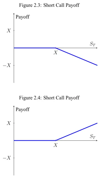
Figure 2.3: Short Call Payoff
X −X X f (x) = x ST Payoff
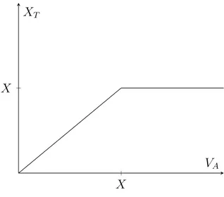
Figure 2.4: Short Call Payoff
X −X X f (x) = x ST Payoff
Its payoff can be represented as
C = −max(ST − K, 0) (2.7)
According to Black and Scholes (1973), a call option price can be found
c = SN (d1) − Ke−rfTN (d2) (2.8) d1 = ln( S K) + (rf + 1 2σ 2)T σ√T (2.9) d2 = ln(KS) + (rf − 1 2σ 2)T σ√T (2.10)
where K is the strike price, rf is the risk-free rate, and S is the underlying asset’s price.
2.2 THE MODEL
2.2.1 Assumptions of the Merton Model
1. Share prices change stochastically and randomly. Merton model assumes that the firm’s asset value is log-normally distributed with constant volatility and follows the Geometric Brownian motion. Hence, it can be inferred from this log-normality assumption is that the returns are also normally distributed.
dVA VA
= µdt+ σAdWt (2.11)
dVA = VAµdt+ σAVAdWt (2.12)
lnVA,t ∼ N (lnVA+ (µ − 1 2σ 2 At), σ 2 At) (2.13) VA,t= VA0e (µ−σ2 A)t+σA √ tWt (2.14) ln(VA,t VA,0 ) ∼ N (µ − 1 2σ 2 At, σA2t) (2.15) where W∼N (0, 1) represents a Wiener process that is a stochastic process. VAis the asset value and µ is the instantaneous drift.
3. The model builds on the assumption that the firm has debt maturing at time T, in the form of a zero-coupon bond.
4. Market interest rates are constant and are known during an option contract.
5. All investors can lend and borrow from the risk-free rate.
6. There is no transaction cost and tax.
7. The structure of the debt of the firm is constant. Debt’s form is a zero-coupon bond, and at the end of the holding period pays principal and interest. Basic firm’s balance sheet can be represented as:
VA,T = VL,T + VE,T (2.16)
where VL,T is debt and is in the form of a zero-coupon bond. The value of a firm is irrespective of the structure capital.
8. The model’s horizon is the 1-year period.
9. The default can be happened at the maturity of the debt, not before.
10. Markets are fully competitive, and there is no arbitrage possibility.
11. Short selling is allowed.
12. Trading is continuous.
13. Shareholders’ wealth is tried to be maximized by management.
14. The firm does not buy back shares issued and not issue senior claims.
2.2.2 Logic Behind Merton Model
In structural methodology, default is an endogenous process, and Merton model pro-vides a theoretical framework that explains which condition will give rise to the default process. Actually, in the original paper, the main aim is to create a model
pricing risky debts. Merton(1974) extended the option pricing method introduced by Black and Scholes(1973) to price risky debt instruments.
In his seminal paper, Merton argued that the equity of the firm could be regarded as the European call option on the firm’s asset value and debtholders have the short position on the firm’s asset value. In this way, the credit risk of the firm can be measured by analyzing the capital structure of the firm. His model then is known as ”structural model” based on the fact that the credit risk of the firm can be explained by analyzing its capital structure. Credit risk of the firm can be priced by looking at the value of the asset and the liability of a firm.
In a typical firm, the asset value will be equal to the sum of equity value and the liability value. Shareholders have limited liabilities on firm and contingent claim on firm assets. They will get after the debtholders’ receivables get paid.
VA= VE + VL (2.17)
Figure 2.5: Default Process
Note. Adapted from ”Modeling Default Risk,” by Crosbie, P., Bohn, J., 2003,Research Report, Moody’s KMV Corporation, p.13.
change the claims on firms as the asset value of the firm changes. In this model, the firm has two options to finance its assets with equity and debt. Under the assump-tion that the default only happens at the maturity date, what the important is the firm value at maturity. So, the probability of default can be defined at this model is the probability that the asset value remains below the liability of the firm at maturity. At figure 2.5, the shaded area that remains the area between default point line(default barrier) and the distribution of asset value is the probability of default. The expected asset value mainly determines the default status at maturity.
In the figure, the line called the default point(default barrier) is the sum of repay-ments of interest rate and principal of the debt within a year. The possible asset value is determined by the lognormal behaviour one of the firms’ value. The figure shows this with the dashed line. However, depending on the asset volatility of the firm, asset value can take different values. This phenomenon is displayed with the possible asset value path line in the figure.
The relative distance between the default barrier(default line)1 and asset value af-fects the probability of default. When asset value gets closer to the default barrier, the credit risk of the firm increases. Also, asset volatility is related to the likelihood of default because when asset volatility is high, then the probability that the asset value falls below the default barrier increases.
According to Merton (1974), under the assumption that the shareholders and debthold-ers are rational, if at the end of the holding period the asset value is less than the liabilities, zero-coupon bond, then shareholders get nothing, debtholders will seize the firm, and they receive the asset value, VA. At the second possible scenario, asset value is more than the liabilities then the residual value that is the difference be-tween the total value of the firm and total liability value goes to shareholders and debtholders receive the total debt. In other words, shareholders have limited lia-bility on the firm. They cannot lose more than the asset value of the firm. When the default happens, debtholders have senior claims on the asset value of the firm, whereas shareholders rank after debtholders. Shareholders’ expected payoff can be
symbolized as: ST = VA,T − XT, if VA,T ≥ XT. 0, otherwise. (2.18)
where ST is the payoff at the expiration date to the shareholder. XT represents the face value of the debt and VA,T is the asset value of the firm.
Figure 2.6: The value of equity at maturity
X X
VA ET
From the debtholder perspective, at the end of the holding period, they will get the asset value of the firm or outstanding debt. In the case, the asset value is less than debt; then the debtholders will get asset value; otherwise, they will receive the debt. This payoff can be represented as:
PT = VA,T, if VA,T ≤ XT XT, otherwise (2.19)
We can rewrite equation 2.19 as:
PT = min(VA,T, XT)
= XT − max(0, XT − VA,T) = VA,T − max(VA,T − XT, 0)
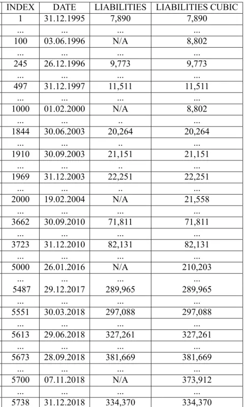
Figure 2.7: The relationship between firm asset value and liabilities at maturity X X f (x) = x VA XT
Risky debt can be shown in two ways, as equation 2.20 above tells us. The value of risky debt is the value of assets minus short position on a call option on firm value. The other equation says that the value of risky debt is the amount of debt minus the short position on the put option. When the firm is in bad situation, shareholders exercise the put option to give the firm to bondholders. At the same time, debtholders also have the option to buy the firm from the shareholders.
The maximum amount that debtholders can take is the amount of debt as long as the firm does not default. The firm that takes debt can pay if the asset value is more than the liabilities. Otherwise, shareholders will transfer the firm’s asset value to debtholder.
Payments caused by the liquidation of asset value is transferred with zero-cost to the debtholders when the firm’s default is realized. At the heart of the model, is the fact that the equity of the firm can be modelled like a European call option. The strike price is the face value of the debt, X, and the maturity is T. This model’s structure is akin to the payoff option. In Merton’s approach, at the maturity, actually, the shareholders will get payment ET
Table 2.1: Payoff Structure Payoff
VA,T < XT VA,T > XT
Shareholder 0 VA,T − XT
Debtholder VA,T XT
This phenomenon proves that the debt structure of a typical firm is a call option that the equity value is the underlying asset, and X is the strike price or the face value of the debt. So the value of the equity resembles the value of a call option. Therefore, the value of equity is:
ET = VA,TN (d1) − Xe−rTN (d2) (2.22) where d1 = ln( VA X ) + (µ + 1 2σ 2 A)T σA √ T (2.23) d2 = ln(VA X) + (µ − 1 2σ 2 A)T σA√T d2 = d1− σA √ T (2.24)
The instantaneous volatility of the equity can be determined by using Ito’s lemma.
E0σE = ∂E
∂AA0σA (2.25)
Call option’s strike price equals to the face of the value of the liabilities. In this setup, the probability of default can be regarded as the probability that the option expires worthless. We are trying to find the probability that the asset’s value of the firm is less than the liabilities(Agarwal and Taffler, 2008).
2.2.3 The Calculation of Probability of Default
The probability of default is that debtholders’ not using the option right at the time maturity T. The implied probability of default can be calculated with the formula presented below. P D = N (−ln( VA X ) + (µ − ψ − 1 2σ 2 AT ) σA √ T ) (2.26)
where V represents the value of the firm, X is the debt of the firm, µ is the expected return of the firm, ψ is the dividend rate defined as total dividend over the total value of the firm given to shareholders, σAis the volatility of the asset and T is the maturity.
Value of assets, the expected return of the firm and volatility of the asset cannot be observed. In equation 2.26, VA and σA can differ in terms of calculation. For example, Hillegeist et al. (2004) find the σAand VAby solving simultaneously 2.27 and 2.28 given below
VE = VAe−ψTN (d1) − Xe−rTN (d2) + (1 − e−ψT)VA (2.27)
σE =
VAe−rTN (d1)σA VE
(2.28)
where VE is the market value of equity, and σAis the standard deviation of the stock returns. In equation 2.27, (1 − eψT) means that shareholders get the dividends, so it decreases the value of equity. But in our model, it is assumed that no dividend is distributed. VAis set initially as VA= VE+ X (2.29) σA= σE VE VE+ X (2.30)
On the other side, Bharath and Shumway (2004) calculate asset volatility in a dif-ferent way σA= VE VA σE + X VA σD (2.31)
Bharath and Shumway (2004) define the relationship between the volatility of debt and the volatility of equity.
σD = 0.05 + 0.25σE (2.32)
Bharath and Shumway (2004) and Hillegeist et al. (2004) differ in picking suitable expected return. Bharath and Shumway (2004) assume the expected return of the firm is the risk-free rate. On the other side, Hillegeist et al. (2004) define the rele-vant return as the past year’s return.
µ = VA,t+ ψ − VA,t−1 VA,t−1
(2.33)
Bharath and Shumway (2004) and Hillegeist et al. (2004) assume the upper boundary for µ as 100%.
Using which µ should be used is entirely arguable an in the literature, we can see many alternatives. For example, Aktan (2011) chooses µ as the log return of implied asset values. Vassalou and Xing (2004) take µ as annual returns of the firms, which can be calculated as the mean of the change in the natural logarithm of the asset value.
Agarwal and Taffler (2008) argue that using past returns as µ is problematic because a distressed firm has more expected return than healthier firm due to carrying high risk.
As stated above, X can be seen as the default barrier for the firm. Vassalou and Xing (2004) determine X as short term plus the half long term debt. Picking X affects the results. This implementation reduces the probability of default due to reduced default barrier.
2.2.4 Determinants of Default
According to Kealhofer (2003), three variables are the main determinants for the default. These are debt level, asset volatility, and asset value.
Merton (1974)’s structural approach implies the liabilities, and asset value of the firm determine the status of default. The primary determinant for the ability to the repayment of the firm depends on the asset value of the firm. When expected asset value increases, we can expect the firm pays more easily its debt.
The value of equity depends on firm value, asset volatility, the face value of debt, maturity, and the risk-free rate. The market value of equity is inversely proportional to the probability of default. When the market value of equity decreases, then the probability of default increases. When the other variables are constant, the increase in the leverage means the firm is riskier. That reduces the distance to default and in-creases the probability of default. Things that rise asset value impact the probability of default positively such as earnings expectations as Chan-Lau et al. (2004) stress, this increases the distance to default. Also, if the expected asset volatility increases, also, the probability of default increases. Likelihood of touching the default barrier rises.
2.2.5 Concept of Distance to Default
Distance to default is how much standard deviation is far away from the default barrier. When the distance to default increases, it implies that the firm gets away from the default. DD is an ordinal measurement. Distance to default can be defined as: DD = ln( VA X) + (µ − 1 2σ 2 A)T σA √ T (2.34)
According to Chan-Lau et al. (2004), the distance to default model permits us to work with the risk-free rate instead of asset value drift. Therefore, µ can be re-placed with the risk-free rate, rf.
DD = ln( VA X ) + (rf − 1 2σ 2 A)T σA√T (2.35)
The relationship between distance to default and the probability of default can be constructed with the equation below.
P D = N (−DD) (2.36)
In the literature, to derive PD, the assumption that the PD is normally distributed is commonly held. Under this assumption, for instance, when we find DD=1, then we can conclude that at maturity, the firm has a PD of 15%. The fact that the proba-bility of default is distributed with standard normal distribution is problematic. For instance, KMV uses its empirical databases to derive PD. Aktan (2011) claims that the financial data, , generally leptokurtic, has leverage effect so, the model’s nor-mality assumption can be replaced with t-distribution that has more fat-tailed.In this case, the probability of default can be represented as:
P D = t(−DD) (2.37)
But the distance to default can be calculated via different methods. For example, as Vassalou and Xing (2004) argue, KMV determines the distance to default as:
DD = VA− DB VAσA
(2.38)
where DB is the default barrier.
2.2.6 Advantages of the Model
When we compared the statistical-based and artificial intelligence models with the Merton model, the fundamental difference is that the latter one is forward-looking. This type of model is more sensitive to changes in the business environment. The former is in nature, static and depends on static financial statements.
In the Merton model, the market reflects all information speedily at securities’ prices. Market-based models are not time-dependent or sample dependent, contrary to acco-unting-based models. The factors that affect credit risk is the same for all samples. The model provides a robust theoretical framework for the default risk contrary to other types such as statistical-based, artificial intelligence models.
The additional confusion related to statistical-based models is about which vari-ables should be added to the analysis. However, for market-based models, there is no question about it.
2.2.7 Limitations of the Model
One of the critics made to Merton Model is that the assumption that the default can only be realized at the maturity date. The basic model does not allow the default be-fore the maturity date. That creates an awkward situation. For example, even until the maturity, the asset value is zero, the firm can be recovered from this situation, and this idea does not capture the real-life condition. So, there are studies that try to relax this assumption. Black and Cox (1976)’s approach allows the firm the de-fault before the maturity. Also, Tudela and Young (2003) create their model based on the Merton model to measure the credit risk of the non-financial firms and relax this assumption, and when asset value fall below default barrier first time, then the default happens.
According to Vassalou and Xing (2004), Merton model assumes that the firm’s debt structure consists of short term debt, long term debt, and equity, so it is simplified. To get close to real life situation, KMV, in Merton’s commercial implementation, the firm’s debt structure is allowed to include convertibles and preferred shares. The second point is that Vassalou and Xing (2004) stress that the Merton model in cal-culating asset volatility is much simpler than the KMV methods that make Bayesian adjustment according to country, industry, size, and so on.
The other problem is that in Merton’s approach, we can predict assuming the prob-ability of default is normally distributed. To overcome this problem, for example, KMV is calculating the probability of default from its own empirical database.
CHAPTER 3 DATA
In a typical firm, we can not directly observe the market value of a firm. For traded companies, we can observe equity value. We can observe the book value of the assets but is often different from the market value. Hence, VA,T cannot be precisely observed. Also, the same issue exists for the asset volatility. We cannot use the asset value to forecast asset volatility. This relationship is derived from option pricing theory. The following section describes how the parameters necessary to calculate. The asset volatility and the asset value of a firm at time T, are obtained or calculated.
3.1 Parameters of the Model
3.1.1 Market Cap
The market value of equity of the firm is calculated as the product of shares price and the number of shares outstanding. Both parameters are obtained from the same database, Bloomberg Terminal. However, the data sequence before 1999 was yearly, after that year, it is obtained quarterly, and it is assumed that no change happens about the number of shares outstanding between periods because of lack of the rel-evant data. Also, market shares outstanding smoothed to average to see the price effect only.
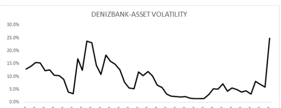
3.1.2 Liability and Default Barrier
As the market cap, the summation of short term and long term debt of the bank is obtained quarterly via Bloomberg Terminal. Since there is no daily debt data, the
cubic spline method is implemented to fill the missing data. The default barrier is picked as the debt of banks, compliant with previous studies.
3.1.3 Risk-Free Rate
Since the period analyzed is too long; unfortunately, there is no unique risk free rate that captures all the period. So, for the period between 1996 and 1998 the risk free rate is assumed to be equal to customer price index published by TUIK and for the period between 1998 and 2005, the risk-free rate is accepted to be equal to the compound return of discounted bond issued monthly by Turkish Treasury is accepted. Also, in some months, since there were more than one issue, the compound return of bond nearest to 1 year is selected as the risk-free rate. Besides, the data is monthly basis. Hence, to get the daily data, the cubic spline method is implemented to fill missing data. For the period after 2005, the yield of the 1-year Treasury Bond is obtained from the Bloomberg Terminal Data daily as daily data.
3.1.4 Maturity
The maturity is accepted as 1-year in parallel with the previous relevant studies.
3.1.5 Drift Rate
As a drift rate, the risk-free rate is picked up in this study. When estimating asset drift, one of the alternatives is to use Capital Asset Pricing Method, but because in our sample horizon is very long, the data availability and reliability are one of the issues, and the model risk can arise. So, the risk-free rate is accepted as the drift rate like Chan-Lau et al. (2004) do.
3.2 Structure of the Data
In this thesis, the distance to default is calculated for banks traded at BIST from 4th quarter of 1996 to last quarter of 2018, by making use of several data sources,
the forecasting power of the Merton model about default and whether it is a good predictor for the crisis is investigated.
Banks used in this thesis to test the theory is illustrated in table 3.1. Table 3.1: Banks used in this study
BANK STATUS TYPE PERIOD
1 YAPI KREDI NON-FAILED COMMERCIAL PRIVATE 1996Q4-2018Q4 2 ALBARAKA NON-FAILED PARTICIPATION PRIVATE 2008Q2-2018Q4 3 DENIZBANK NON-FAILED COMMERCIAL PRIVATE 2005Q4-2018Q4 4 FINANSBANK NON-FAILED COMMERCIAL PRIVATE 1997Q4-2018Q4 5 FORTIS NON-FAILED COMMERCIAL PRIVATE 1997Q4-2010Q4 6 VAKIFBANK NON-FAILED COMMERCIAL STATE 2007Q1-2018Q4 7 ISBANK NON-FAILED COMMERCIAL PRIVATE 1996Q4-2018Q4 8 GARANTI NON-FAILED COMMERCIAL PRIVATE 1996Q4-2018Q4 9 HALKBANK NON-FAILED COMMERCIAL STATE 2008Q2-2018Q4 10 TOPRAKBANK FAILED COMMERCIAL PRIVATE 1999Q2-2001Q2 11 AKBANK NON-FAILED COMMERCIAL PRIVATE 1996Q4-2018Q4 12 TEB NON-FAILED COMMERCIAL PRIVATE 2001Q2-2015Q2 13 TSKB NON-FAILED DEVELOPMENT PRIVATE 1996Q4-2018Q4 14 DEMIRBANK FAILED COMMERCIAL PRIVATE 1996Q4-1999Q4 15 TUTUNBANK FAILED COMMERCIAL PRIVATE 1996Q4-1999Q4 16 ASYA KATILIM FAILED PARTICIPATION PRIVATE 2007Q2-2015Q3
The sample consists of 16 banks operated between 1996 and 2018 at BIST Banking Index. 4 banks are captured by TMSF, and these banks are classified as failed banks. Others are labelled as non-failed banks. Two of them are participation banks, one of them is development bank and others can be classified as commercial banks. Our sample size differs each year because of data availability and the status whether it is traded at BIST or not. For example, ICBC and ESBANK are not included in our sample since we did not reach reliable data about them. Table 3.2 shows the sample size for each year examined.
3.2.1 Steps to Follow
I created a sheet at Excel for each quarter that captures last one year data. The neces-sary variables for the model are market capitalization, book liabilities, risk-free rate,