Hourly electricity demand forecasting using Fourier analysis with feedback Ergun Yukseltan, Ahmet Yucekaya*, Ayse Humeyra Bilge

(1)

Energy Strategy Reviews 31 (2020) 100524

Available online 21 July 2020

Hourly electricity demand forecasting using Fourier analysis with feedback

Ergun Yukseltan , Ahmet Yucekaya

*

_{, Ayse Humeyra Bilge}

Industrial Engineering Department, Kadir Has University, Istanbul, Turkey

A R T I C L E I N F O Keywords:

Time series analysis Prediction Forecast Fourier series Modulation Feedback A B S T R A C T

Whether it be long-term, like year-ahead, or short-term, such as hour-ahead or day-ahead, forecasting of elec-tricity demand is crucial for the success of deregulated elecelec-tricity markets. The stochastic nature of the demand for electricity, along with parameters such as temperature, humidity, and work habits, eventually causes de-viations from expected demand. In this paper, we propose a feedback-based forecasting methodology in which the hourly prediction by a Fourier series expansion is updated by using the error at the current hour for the forecast at the next hour. The proposed methodology is applied to the Turkish power market for the period 2012–2017 and provides a powerful tool to forecasts the demand in hourly, daily and yearly horizons using only the past demand data. The hourly forecasting errors in the demand, in the Mean Absolute Percentage Error (MAPE) norm, are 0.87% in hour-ahead, 2.90% in day-ahead, and 3.54% in year-ahead horizons, respectively. An autoregressive (AR) model is also applied to the predictions by the Fourier series expansion to obtain slightly better results. As predictions are updated on an hourly basis using the already realized data for the current hour, the model can be considered as reliable and practical in circumstances needed to make bidding and dispatching decisions.

1. Introduction

Demand forecasting has always played an important role in capacity and transmission planning, generation planning, and pricing. Also, the liberalization and privatization of power markets have increased the importance of demand or load estimation as market success rates are largely related to their accuracy.

Demand forecasting has different aspects in different forecast hori-zons. For example, for capacity planning, long-term estimation of the total demand as a function of economic or demographic parameters is needed. On the other hand, short-term (hourly) estimates are necessary for the effectiveness of day-ahead markets. Short-term variations have a "regular" component depending on daily routine and seasonal effects. Exceptional conditions (extreme weather conditions) and exceptional events (holidays, sporting events) cause "irregular" variations that affect and change this pattern. The prediction of the "regular" component of the hourly demand is important for the planning of the day ahead market in the long run, that is, on a horizon throughout the years. Also, it is desirable to adopt these estimates to rapidly changing conditions efficiently and reliably.

A modulated Fourier series expansion is used in order to take into account the variability in the amplitudes of the daily variations, without

using any climatic information in Ref. [1]. This method is applied to the Turkish power market data for the period 2012–2017 to predict hourly demand over the 1-year horizon within a 5% error margin in the Mean Absolute Percentage Error (MAPE) norm. The key fact for achieving such a low prediction error is the fact that in Turkey, household elec-tricity is used mainly for illumination, hence consumption patterns follow an annual cycle and they can be predicted in terms of the har-monics of the annual and daily variations.

In this paper, this prediction scheme is supplemented with a 1-h ahead forecast using “feedback” [2]. In this scheme, if there is an un-usual event causing below or above average consumption, the discrep-ancy between the actual consumption and the prediction is used to modify the prediction for the next hour. In cases where the typical duration of the irregular events is long compared to the sampling period (here 1 h), this approach turns out to be successful in reducing the forecast error.

In addition to linear models and time series methods, alternative heuristic methods such as Artificial Neural Networks (ANN), Genetic Algorithms (GA), Support Vector Machines (SVM), and Particle Swarm Optimization (PSO) and other numerical methods are common ap-proaches used for the electricity demand forecasting. A detailed analysis of the literature on forecasting methods is given in Ref. [1].

* Corresponding author.

E-mail address: [email protected] (A. Yucekaya).

Contents lists available at ScienceDirect

Energy Strategy Reviews

journal homepage: http://www.elsevier.com/locate/esr

https://doi.org/10.1016/j.esr.2020.100524

(2)

As opposed to deterministic models, stochastic effects are taken into account by time series methods such as Autoregressive Moving Average (ARMA) or Autoregressive Integrated Moving Average (ARIMA) models. As periodicities in the data appear as correlations at the corresponding period, these models can represent periodic variations, but their main advantage is the representation of short-term correlations and the modelling of additive noise.

The effects of weather variables on electricity load are far from being simple, as discussed in several research papers. For example, Apadula et al., present a study that analyses the effect of climate parameters on the electricity demand for Italy, showing that the information on tem-perature, relative humidity, wind velocity, and cloudiness increase forecast accuracy [3]. On the other hand, McCulloch and Ignatieva claim that including different climatic parameters to a model can create collinearity problems hence they only use temperature in their model [4]. In Refs. [5], the authors show that electricity consumption due to cooling needs continues even after the high temperatures return to normal due to the fact that the buildings kept their heat capacity. All these results show that the effects of weather conditions on electricity consumption are quite complicated even “nonlocal” as a function in time, in the sense that not only the present values of the regressors but their past values also affect the current electricity demand. In the pro-posed approach, these effects are taken into account by the modulated Fourier expansion and by the feedback mechanism.

As examples of general forecast models, in Ref. [6], the authors use weather scenarios to forecast short-term electricity demand for 1–10 days ahead. In Ref. [7,8] the researchers use statistical modelling to analyse the influence of temperature on load forecasting in Italy, both at the national and regional level, using historical load data. In Ref. [9], different load profile patterns are used to analyse the effect of weekly, daily, and seasonal cycles. The effects of climatic parameters on elec-tricity demand are studied in Ref. [10,11], and [12]. The same topic is also studied in Ref. [13] where it is shown that for Prague, Czech Re-public, the sunshine duration is more important than outside temperatures.

As seen from the remarks above, temperature data alone is insuffi-cient to give satisfactory results because other climatic parameters such as relative humidity and cloudiness affect feeling temperature and consumer behaviour. Also, as it is not easy to collect detailed and reli-able weather data for every consumption region, methods that use only past data are of practical importance.

The electricity demand in the holidays is nonstandard. This issue is taken into account in a model for hourly electricity demand, where data for the holidays is replaced with an interpolation of demand for the before and after holiday periods in an effort to smooth the demand data for better forecasting results [14]. A similar approach is also adopted in Ref. [1] as well as in the present one, as part of the pre-processing scheme.

ARMA type methods are successful in following trends that are relatively slow compared to the sampling rate. Thus, they are suitable for long-term slow trends such as the ones related to economic growth, etc., or short-term trends such as hourly variations in a day. For example, in Ref. [15], future demand is predicted using an ARIMA model and a profit function is developed as an objective. In Ref. [16], the researchers propose an econometric modelling approach for the long-term forecasting of hourly electric consumption in local areas, using data from the Danish market and estimate load profiles of the transmission operator. In another study, the authors use Artificial Neural Networks and ARIMA models to calculate the load and examine local forecast uncertainty to show high risk in different periods and evaluate daily value at risk [17].

In the literature, time series methods are also combined with other heuristic approaches. For example, in Ref. [18] the author studies En-gland and Wales electricity demand data in the half-hour period data series and applies the Holt-Winters method for different periods with AR model. In Ref. [19], the authors show that the "PSO optimal Fourier

method" corrects seasonal ARIMA forecast results, and apply it to the Northwest China electrical network, showing that the combined model’s forecasting accuracy is higher than that of single-season ARIMA. A new type of neural network method to forecast short-term electricity demand is presented in Ref. [20] where it is shown that its performance is better than ARIMA. In Ref. [21], the authors use nonparametric functional methods to forecast the next day’s electricity demand of Spain and show that the results are competitive with other methods, including ARIMA. A functional approach is proposed in Ref. [22] to forecast electricity de-mand by modelling variations in a week while data from the Turkish power market is used to validate the accuracy of the model. In Ref. [23] the authors use statistical analysis methods to forecast short-term de-mand and show that the proposed method can outperform ARIMA. [20].

In this paper, the linear model proposed in Ref. [1] is upgraded, which consists of a Fourier series expansion in which workdays and weekends form two nearly independent sets of variations. As for the pre-processing, based on a comprehensive analysis of daily variation patterns, a coding system is used to identify days as “religious holiday”, “official holiday”, “New Year’s Eve”, “weekends” and “weekdays”. Knowing the characteristics of these days, the prediction is adjusted by Fig. 1. Daily data for 2012–2017 with daylight savings time correc-tion removed.

(3)

Energy Strategy Reviews 31 (2020) 100524

certain percentages. After obtaining predictions over various time ho-rizons, the hourly predictions are updated (over any time horizon) by a 1-h ahead forecast, by feeding back the prediction error multiplied by a constant k. This constant parameter is optimized and with this simple method, a forecast error of less than 1% MAPE is achieved. In order to improve the mechanism for updating the predictions, an AR model is applied to the residual of past data and the linear model.

In Section 2, an overview of the Turkish Power market, the data used for the validation of the model, and a discussion of the structure of the daily variation curves and the effect of exceptional events are presented. Then, a linear regression model, using low and high-frequency har-monics and their interaction as modulated waves are proposed. Fore-casting for 1-year and 1-day horizons are presented in Section 3. In Section 4, various schemes for the forecasting of the demand using feedback methodology are used. Section 5 presents discussion and Section 6 presents the conclusion and suggestions for future directions respectively.

2. Data processing and model formulation

In Turkey, household electricity consumption is approximately 68%, and the electricity is not commonly used (about 8.6%) for heating in winter but it is used for cooling needs in summer [24]. Another distinctive feature of the data for Turkey is the demand pattern during religious holidays as discussed in the sequel.

As can be seen from Figs. 1 and 2, electricity consumption has a trend of increase, a strong seasonality, with high consumption periods in winter and summer and low consumption periods in spring and fall (Fig. 1a). Furthermore, consumption is lower on weekends compared to

weekdays (Fig. 1b). Also, daily variations have higher amplitudes in periods of high average consumption (Fig. 2). Electricity consumption for heating and cooling purposes has a strong dependence on tempera-ture, or more precisely on deviations from comfortable temperatures. As climate conditions may display considerable variations from seasonal averages, it is hard to make predictions over a long term horizon. Thus, in regions where electricity is used for heating, the modulated Fourier Series Expansion is not expected to achieve satisfactory performance.

Nonindustrial electricity can be used for illumination, cooling, and heating. If cooling and heating are negligible, data is more regular, and the highest consumption occurs in winter due to illumination needs. Cooling and heating increase consumption in winter and summer respectively and cause irregularities in the consumption waveforms.

The hourly demand and consumption data for the whole country are provided by the system operator. These data include market prices, hourly imbalances, and other related information, without any demand type or region segregation. In Fig. 1, an overview of daily averages of the data for the years 2012–2017 is presented. Data displayed in this figure have been pre-processed to correct irregularities due to switching to daylight saving time, by removing zero consumption and double con-sumption values at these dates. The difficulties associated with daylight savings time are not that simple, because this sudden change in the illumination period hinders the success of the prediction for some period following the change, as discussed in detail in Ref. [1].

In Fig. 1a, the low-demand periods correspond to two religious holidays of durations of 3 and 4 days respectively. These holidays are determined according to the lunar calendar and they are shifted back by 10 days each year in which most factories stop their operations. As a result of a qualitative observation concerning holiday periods, it is Fig. 2. Typical daily load profiles in winter, spring, summer, and fall.

(4)

concluded that the consumption pattern for the religious holidays is very specific and should be treated separately. Typical weekday variations in winter, summer, spring, and fall are shown in Fig. 2.

Due to the illumination needs, nonindustrial electricity consumption increases in winter. The need for illumination decreases in summer but consumption increases again because of the extra demand for cooling. In addition to base level differences, the amplitudes of daily variations are different in each season. This fact is identified as the modulation of the high frequency (daily) variations with low frequency (seasonal) variations.

2.1. Methodology and modelling

Fourier series expansion is a powerful tool for the modelling of pe-riodic signals. If a function f(t) is pepe-riodic and its period is T, then the Fourier series for f(t) is an infinite sum of sine and cosine functions with periods T/n. It is known that under mild assumptions, the Fourier series converges to f(t) at points of continuity. The sinusoids whose frequencies are multiples of the basic frequency 1/T, are called the “harmonics” of the main variation. If one works with sampled data, that is samples of f (t), at time intervals Δt, then, the original signal can be reconstructed from the sampled data, provided that it contains harmonics whose fre-quencies are less than 2/Δt. This means that, if one works with hourly samples of the data, only variations with periods greater than 2 h can be modelled.

A glance at the electricity consumption data shows that there are 3 systems of variations, the “seasonal variation” with the main period 1 year, the “weekend effect” with the main period of 7 days, and the diurnal variation of main period 24 h. The number of harmonics for each system of periodicities is chosen to be high enough to reproduce the essential features of the basic shape. The restriction on the upper bound for these harmonics comes in the diurnal variation; as the smallest period that can be present in the expansion is 2 h, only 12 harmonics are included.

An expansion into a sufficiently high number of harmonics captures the shapes of the variations, but the amplitude of the variation changes throughout a year. In order to take into account this fact, “modulation”

is used, which is a standard technique in signal processing. Modulation consists of multiplying the low frequency signal (usually an audio signal) with a high frequency signal (called the carrier). The high fre-quency signal is broadcast and carries the information content of the low frequency signal. In the proposed approach, products of low and high frequency variations are added as regressors to replicate the change in the amplitude of the high frequency variations throughout the year.

The final ingredient of the proposed method is “feedback”. This is a standard tool in control engineering that consists of “feeding” the de-viation from the desired output as an input to a system. The modulated Fourier series expansion reproduces seasonal and illumination related variations quite faithfully, without using any external parameters. Some of the remaining variations are stochastic but the majority are due to foreseeable events. In this case, cooling needs that are arising from extreme weather conditions constitute the main cause of irregular events in consumption. The typical duration of weather-related phe-nomena is a few days; hence they may be considered as trends spanning several sampling periods. For example, temperatures above and below seasonal averages increase heating and cooling needs. At the onset of these events, actual consumption is higher than predicted by the modulated Fourier series expansion. In the feedback scheme, once a deviation from the predicted value is observed, the forecast is updated. This allows following the trend up to the reversal. The method has the advantage of being simple and not requiring any external information but introduces errors at trend reversals. Including weather projections as regressors would of course remediate this drawback and would result in sharper estimates as in Ref. [25], but it is not applied in the present work.

As data consist of hourly samples, the basic unit of time is hour and regressors are represented as column vectors with length equal to the total duration of the observation period in hours. The hourly electricity demand is denoted by S. A constant vector (denoted by 1) and a linear term (denoted by t) to take into account the trend in the data are used. Periodic variations are the n’th harmonics of sinusoidal functions with periods 1 year, i.e, (364x24)/n hours (denoted by Xn), m’th harmonics of

1 week i.e, 7 � 24 h (denoted by Zm), and the k’th harmonic of 1 day i.e,

24 h (denoted by Yk). The regressors that represent the modulation of

(5)

the high-frequency variations (Yk) by the low-frequency variations (Xn)

is included by the component-wise product of the corresponding vectors, denoted as XnZm and XnYk. These regressors are arranged as the columns

of a matrix F;

F ¼ ½1 t X1X2 XN Z1Z2 ZM X1Z1 XNZM Y1Y2 YK X1Y1 XNYK� (1) The number of regressors should be large enough to capture the main features of the data but over-specification should be avoided. In addi-tion, by the sampling theorem, the shortest allowable period is 2 h. By taking into account these considerations, a model is built that uses 96- time regressors to represent sinusoidal variations and 160 regressors to implement modulation effects. The coefficient vector a and model vector y are calculated as below.

a ¼ ðFt_FÞ 1

Ft_S ₍₂₎

y ¼ Fa (3)

In the assessment of the performance of the model, the Root Mean Square Percentage Error (RMSPE) and Mean Absolute Percentage Error (MAPE) are used. If Sh and yh are the actual demand and the forecast

demand for hour h, then RMSPE and MAPE can be defined as: RMSPE ¼ ffiffiffiffiffiffiffiffiffiffiffiffiffiffiffiffiffiffiffiffiffiffiffiffiffiffiffiffiffiffiffiffiffi 1 N XN h ðyh ShÞ2 S2 h v u u t ₍₄₎ MAPE ¼100 N X h 1N � �ðyh ShÞ2 � � S2 h (5)

where N is the total number of estimated values.

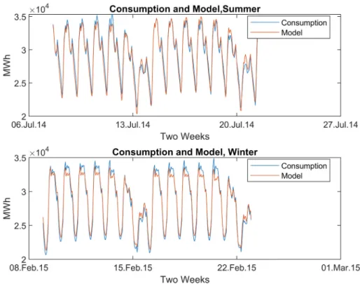
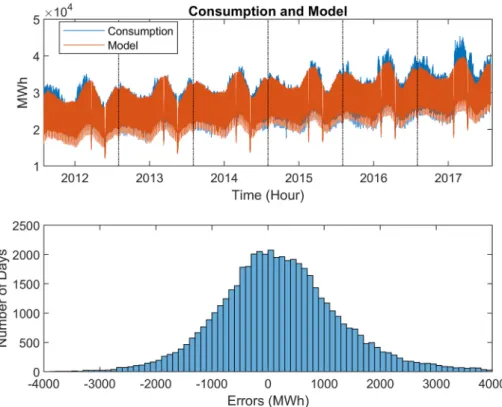
Fig. 3 provides a comparison of the actual data and the proposed model for typical 2-week periods in winter and summer. It is clear that not only the amplitude but also the shape of the periodic variations for weekdays, weekends, summer and winter are different. Fig. 4 shows the forecasted and actual data for the analysis period. The modelling errors for the whole 6-year period are respectively 4.13% (RMSPE) and 2.97% (MAPE).

In Fig. 4 a-b, the actual and forecasted demand values, the change of the modelling error through the analysis period, and the histogram of the errors in MWh are presented. It is worth mentioning that the de-viations from the actual values increase in winters and summers as ex-pected. This can be interpreted as the effect of climatic parameters and their effect on the demand.

3. Prediction over 1-year and 1-day horizons

In order to assess the performance of the model on future data, the time axis is split into “past” (t1) and “future” (t2) with a corresponding

splitting of the regressor functions. Then a corresponding splitting of the matrix F, into F1 and F2 created. In order to make a prediction, F1 is used

to compute the coefficient vector a but F2 is used to compute the model

vector y2 as shown in equation (6). Usually, the prediction error is larger

than the modelling error; the forecast accuracy of the models for the annual and daily forecast periods are presented in the following sections. a1¼ F1tF1

� 1 Ft

1S1 y2¼F2a1 (6)

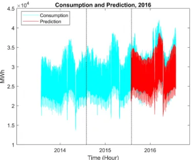
3.1. Prediction over a 1-year horizon

The model is applied to a 2-year observation period, and the model is used based on this observation period to make an hourly prediction for the next year. In other words, hourly data for three years is used in forecasting process of which two years are for learning and one year is for validation. Therefore, forecasts can be obtained just for the years 2014, 2015, 2016, and 2017. This long-term prediction is necessary to Fig. 4. a. Data and model for the period 2012–2017, b. histogram (lower panel).

Table 1

Errors for hourly prediction over a 1-year horizon.

Error Types/Years 2014 2015 2016 2017

RMSPE 4.96% 4.46% 5.45% 5.54%

MAPE 3.69% 3.10% 3.75% 3.62%

(6)

make large scale planning for the electricity market. The prediction errors for each year are given below in Table 1.

Fig. 5 displays the forecast values and the actual values for 2016 as an example of the training and validation periods.

3.2. Prediction over a 1-day horizon

The same method is adopted and the model parameters are updated using data of the previous 2-year period to predict the next day and this process is repeated for each day. This can be interpreted as viewing data over a sliding observation window of a length of two years (2x52 � 7 days) and applying the prediction with a 1-day roll-over period. Every day, the model is updated using the latest available data. Fig. 6 presents the day ahead forecast and the histogram of the error distribution for the

day ahead forecast model.

The same methodology can be used for the day-ahead predictions. RMSPE and MAPE values for the day-ahead prediction errors are given below in Table 2. Note that the model coefficients are recalculated at each hour based on the past 2 years’ data. The approach is practical for power companies as the moving window dynamically rearranges its coefficients and returns better results compared to the prediction over a 1-year horizon, as seen in Table 2.

4. 1-Hour ahead forecast using feedback

In the previous section, the results for the prediction of the hourly consumption over 1-year and 1-day horizons, in terms of a modulated Fourier expansion are presented. The discrepancies between the actual consumption and daily prediction are mainly due to weather conditions or unplanned extended holidays. Although it would be possible to incorporate climatic information into the model, adopt a data- independent approach adoption is preferred. In this section, a 1-h ahead forecast for consumption is obtained as a correction term to the 1-day horizon predictions. This simple approach is the “feedback” method that consists of adding a multiple of the prediction error for the previous hour as a correction term.

In order to determine the best feedback parameter, the model is run with feedback parameters in a certain range and the prediction errors are calculated. The value leading to the lowest MAPE and RMSPE values is chosen as the feedback parameter. The feedback parameter based on the full 6 year period is found to be k ¼ 0.96, as shown in Fig. 7a. In order to study the time variation of the feedback coefficient, this pro-cedure is repeated every quarter and the resulting feedback coefficients Fig. 5. Consumption data and prediction over a 1-year horizon for 2016.

Fig. 6. a. Data and day-ahead prediction for the period 2012–2017 (upper panel) and c. histogram (lower panel). Table 2

Errors for hourly prediction over the 1-day horizon.

RMSPE 3.01% 3.10% 3.42% 3.52%

(7)

are plotted on Fig. 7b, together with their error bounds. The forecast values, zi are defined as

zðnÞ ¼ yðnÞ þ k ðSðn 1Þ yðn 1ÞÞ n > 1 (7)

where S and y are the observed and predicted values respectively and k is the feedback coefficient.

The application of feedback decreases forecast error to about 1% MAPE as shown in Table 3 a1 ¼ F1t � F1-1 � F1t � S1a1 ¼ F1t � F1-1 � F1t � S1.

4.1. AR models

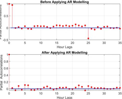
A more sophisticated approach for error correction is to apply an autoregressive model to the difference between data and day-ahead prediction. The analysis of this time series shows that partial autocor-relation function, shown in Fig. 8, displays a strong correlation at lag 1 and less accentuated correlations at lags that are related to daily variation.

In the autoregressive model AR (1,24,25) the coefficient of the lag 1 regressor is c1 ¼0.900, which is close to the value found by the best feedback coefficient, k ¼ 0.96. Coefficients for 24- and 25-h lags are c24

¼0.476 and c₂₅¼ 0.440 respectively. The AR (1,24,25) model for the forecast z(n) is given by

zðnÞ ¼ yðnÞ þ c1hðn 1Þ þ c24hðn 24Þ c25hðn 25Þ n > 25 (8) y(n) is the day-ahead linear regression model, h(n) differences between observation and prediction (S(n)-y(n)). The autoregressive model applied to the difference between the data and the day-ahead prediction improves the simple feedback by adding correlations at lags that are multiples of 24 h, as shown in Table 4.

The results of the forecasts with feedback are shown in Fig. 9. One can see that the histogram of errors shows that the spread has been decreased significantly.

The residuals with and without feedback are presented in Fig. 10 in which the residual for day-ahead and hour-ahead predictions are shown. One can see that the residual has a lower amplitude in general but displays certain high peaks. This is an unavoidable feature of the feed-back mechanism because it introduces twice the error with trend re-versals. A close up for data, day-ahead prediction and 1-h ahead forecast for a typical week period are shown in Fig. 11.

The results that compare the performance of the models are sum-marized in Table 5 below.

5. Discussion

The regressors are supplemented by a modulation of the high- frequency components using seasonal harmonics. With the inclusion of modulated regressors, prediction within an error margin of 3% in MAPE over a 1-year horizon is achieved, without using any climatic informa-tion. The Feedback methodology is used to correct the prediction error and obtain a 1-h ahead forecast within 1% MAPE margin, without using any external parameters as regressors.

As can be seen in Table 5, the forecasting accuracy is improved approximately %70 with feedback correction and also it is very close to the AR (1,24,25) model. The power of the proposed model against prevalent methods in literature is making forecasts using only con-sumption data and calendar information and the flexibility of the fore-cast horizon. The impact of climatic parameters on electricity demand has been a subject of many researches in the literature [2–13]. The pa-rameters such as temperature, humidity, solar radiation, and cloudiness might affect the demand. The researches that use methods such as ARIMA and AR have been found effective in predicting the demand and they were applied to forecast the demand [15–20]. However, such models in literature have been used to forecast only short-term demand. On the other hand, the proposed model provides quality short term forecast similar to the common models in literature and also long term forecast that is important to get an idea for future consumption pro-jection. Furthermore, there is no need for any other data such as tem-perature, humidity, or heating-cooling degree day. The authors use weather parameters to improve electricity load forecasting accuracy in Ref. [9,25], and [26]. A detailed collection of case studies and demand forecasting models is also provided in Refs. [27]. However, for aggregate planning, collecting weather parameters are not easy and practical for countries like Turkey due to the large land area. The data measurements may be different even in weather stations that are placed in the same Fig. 7. (a) Best feedback coefficient based on 6 years data; (b) Best feedback

coefficients based on 3 month periods. Table 3

Errors for hourly prediction over the 1-day horizon when applying feedback.

RMSPE 1.11% 1.12% 1.18% 1.33%

MAPE 0.83% 0.84% 0.89% 0.94%

(8)

city. Therefore, collecting and processing such data is difficult and in-crease complexity.

In addition to seasonality, consumption during weekdays and weekends are different, as seen in Fig. 12. This complicates the appli-cation of SARIMAX type models and special techniques are needed [23]. In the proposed approach, the periodic variations are taken into account by the Fourier series expansion. In the literature, demand forecasting for Fig. 8. The partial autocorrelation function for the difference between data and the day-ahead prediction, before and after applying AR modelling. Table 4

Errors for hourly prediction over the 1-day horizon when applying AR model.

RMSPE 1.06% 1.09% 1.06% 1.20%

MAPE 0.72% 0.71% 0.72% 0.77%

(9)

separate days using specific methods are also used [28]. A similar approach was adopted in earlier attempts but as the results were not found satisfactory, it was abandoned. The MAPE values of each day distributed between 3.43% and 4.19% which are greater than the

modelling error of the proposed model in this paper.

Household electricity consumption is dominated by illumination, heating, and cooling needs; hence it has strong periodic components whose amplitudes depend on climatic conditions. At all prediction ho-rizons, the stochastic nature of the demand has to be taken into account and appropriate tools have to be used. Holidays and special events are irregular but predictable events that affect electricity consumption to a great extent. In particular, in the Islamic world, religious holidays are determined according to the lunar calendar and they start 10 days earlier each year. These types of problems require special methods for dealing with special days and events.

As a further discussion of temperature effects, a scatter plot of elec-tricity consumption for the years 2012–2017 versus temperature is Fig. 10. Residuals for day-ahead prediction and 1-h ahead forecast.

Fig. 11. Close up for 1-h ahead forecast including actual, day-ahead prediction. Table 5

Comparison of errors after applying feedback to the day-ahead prediction through 2014–2017.

Error/Forecast Without Feedback With Feedback With AR

RMSPE 4.38% 1.30% 1.11%

MAPE 2.93% 0.87% 0.73%

Fig. 12. Average daily curves for the years 2012–2017. E. Yukseltan et al.

(10)

presented in Fig. 13. The data is arranged using 6-h intervals. It can be seen that especially during working hours, electricity consumption is more sensitive to high temperature than low temperature as pointed before as more electricity is used for cooling necessities in summer than for heating in winter.

6. Conclusion

Electricity demand forecasting plays a key role in power companies as they need to develop long- and short-term strategies. In this work, aggregate electricity demand for the period of 2012–2017 was analysed and a linear regression model in terms of the harmonics of the daily, weekly and seasonal variations and a modulation by seasonal harmonics was developed. A feedback mechanism and an autoregressive part to forecast the demand are added to forecast. The methodology calculates and updates the feedback coefficient at each step of the moving window and forecasts demand based on the new parameter. Then a better rep-resentation of the actual variability is included in the model and hence the forecast accuracy is improved.

The proposed method is able to forecast the hourly demand with a 0.87% MAPE with feedback and 0.73% MAPE with AR included from 2014 to 2017. The results are quite satisfactory for the electric power demand forecasting literature as well as the industry.

The computation time is an important parameter to consider as forecasting is a daily activity. The computations are performed in intel core The proposed approach was implemented using Matlab and com-putations are performed with intel core i7-377T having 2.5 GHz of

processing speed and 8 GB Ram. The long-term forecasting took 1.35 s, daily prediction for 4 years took 153.35 s and the entire analysis including the creation of visual elements took 227 s.

The proposed model is applicable to the electricity demand data for any country, provided that special days such as holidays are identified and treated separately. Nevertheless, better performance is expected to occur in cases where the usage of electricity for heating purposes is limited.

Funding

This research received partial funding from Kadir Has University, Turkey.

Declaration of competing interest

The authors declare no conflict of interest.

CRediT authorship contribution statement

Ergun Yukseltan: Methodology, Validation, Formal analysis,

Investigation, Writing - original draft, Writing - review & editing, Su-pervision. Ahmet Yucekaya: Conceptualization, Validation, Formal analysis, Investigation, Writing - review & editing, Supervision. Ayse

Humeyra Bilge: Methodology, Validation, Formal analysis,

Investiga-tion, Writing - original draft, Writing - review & editing, Supervision. Fig. 13. Temperature and Consumption Comparison in different hours (2012–2017).

(11)

Acknowledgments

The authors acknowledge the financial assistance from the Kadir Has University, Turkey for the support to energy and power market research.

References

[1] E. Yukseltan, A. Yucekaya, A.H. Bilge, Forecasting electricity demand for Turkey:

modeling periodic variations and demand segregation, Appl. Energy 193 (2017)

287–296.

[2] A.H. Bilge, Y. Tulunay, A novel-on-line method for single station prediction and

forecasting of ionospheric critical frequency for F2 1 hour ahead, Geophys. Res.

Lett. 27 (2000) 1383–1386.

[3] F. Apadula, A. Bassini, A. Elli, S. Scapin, Relationships between meteorological

variables and monthly electricity demand, Appl. Energy 98 (2012) 346–356.

[4] J. McCulloch, K. Ignatieva, Forecasting high frequency intra-day electricity demand using temperature, SSRN Electr. J. (2017), https://doi.org/10.2139/

ssrn.2958829.

[5] C. Crowley, F.L. Joutz, Hourly electricity loads: temperature elasticities and

climate change, in: Presented at the 23rd US Association of Energy Economics

North American Conference, Mexico City October 19-21, 2003.

[6] J.W. Taylor, Short-term electricity demand forecasting using double seasonal

exponential smoothing, J. Oper. Res. Soc. 54 (8) (2003) 799–805.

[7] M. De Felice, A. Alessandri, P.M. Ruti, Electricity demand forecasting over Italy:

potential benefits using numerical weather prediction models, Elec. Power Syst.

Res. 104 (2013) 71–79.

[8] M. De Felice, A. Alessandri, F. Catalano, Seasonal climate forecasts for medium-

term electricity demand forecasting, Appl. Energy 137 (2015) 435–444.

[9] P. Lusis, K.R. Khalilpour, L. Andrew, A. Liebman, Short-term residential load

forecasting: impact of calendar effects and forecast granularity, Appl. Energy 205

(2017) 654–669.

[10] S.M. Islam, S.M. Al-Alawi, K.A. Ellithy, Forecasting monthly electric load and

energy for a fast growing utility using an artificial neural network, Elec. Power

Syst. Res. 34 (1) (1995) 1–9.

[11] C.L. Hor, S.J. Watson, S. Majithia, Analyzing the impact of weather variables on

monthly electricity demand, IEEE Trans. Power Syst. 20 (4) (2005) 2078–2085.

[12] M.A. Momani, Factors affecting electricity demand in Jordan, Energy Power Eng. 5

(2013) 50–58.

[13] M. Ba�sta, K. Helman, Scale-specific importance of weather variables for

explanation of variations of electricity consumption: the case of Prague, Czech

Republic, Energy Econ. 40 (2013) 503–514.

[14] S. Brubacher, G. Wilson, Interpolating time series with application to the

estimation of holiday effects on electricity demand, Applied Statistic 25 (2) (1976)

107–116.

[15] J. Niu, Z.-h. Xu, J. Zhao, Z.-j. Shao, J.-x. Qian, Model predictive control with an on-

line identification model of a supply chain unit, J. Zhejiang Univ. - Sci. C 11 (5)

(2010) 394–400.

[16] F.M. Andersen, H.V. Larsen, R.B. Gaardestrup, Long term forecasting of hourly

electricity consumption in local areas in Denmark, Appl. Energy 110 (2013)

147–162.

[17] K.L. Lo, Y.K. Wu, Risk assessment due to local demand forecast uncertainty in the

competitive supply industry, IEE Proc. Generat. Transm. Distrib. 150 (5) (2003)

573–581.

[18] J.W. Taylor, R. Buizza, Using weather ensemble predictions in electricity demand

forecasting, Int. J. Forecast. 19 (1) (2003) 57–70.

[19] Y. Wang, J. Wang, G. Zhao, Y. Dong, Application of residual modification approach

in seasonal ARIMA for electricity demand forecasting: a case study of China,

Energy Pol. 48 (2012) 284–294.

[20] Y. Ren, P.N. Suganthan, N. Srikanth, G. Amaratunga, Random vector functional

link network for short-term electricity load demand forecasting, Inf. Sci. 367

(2016) 1078–1093.

[21] J.M. Vilar, R. Cao, G. Aneiros, Forecasting next-day electricity demand and price

using nonparametric functional methods, Int. J. Electr. Power Energy Syst. 39 (1)

(2012) 48–55.

[22] Ü.B. Filik, €O.N. Gerek, M. Kurban, A novel modeling approach for hourly

forecasting of long-term electric energy demand, Energy Convers. Manag. 52 (1)

(2011) 199–211.

[23] Y. Chakhchoukh, P. Panciatici, L. Mili, Electric load forecasting based on statistical

robust methods, IEEE Trans. Power Syst. 26 (3) (2010) 982–991.

[24] V.S¸. Ediger, G. Kirkil, E. Çelebi, M. Ucal, Ç. Kentmen-Çin, Turkish public

preferences for energy, Energy Pol. 120 (2018) 492–502.

[25] N. Elamin, M. Fukushige, Modeling and forecasting hourly electricity demand by

SARIMAX with interactions, Energy 165 (B) (2018) 257–268.

[26] Y. Wang, J.M. Bielicki, Acclimation and the response of hourly electricity loads to

meteorological variable, Energy 142 (2018) 473–485.

[27] F. Riva, A. Tognollo, F. Gardumi, E. Colombo, Long-term energy planning and

demand forecast in remote areas of developing countries: classification of case studies and insights from a modelling perspective, Energy strategy reviews 20

(2018) 71–89.

[28] S. Khan, N. Javaid, A. Chand, A.B.M. Khan, F. Rashid, I.U. Afridi, Electricity load

forecasting for each day of week using deep CNN, in: Workshops of the International Conference on Advanced Information Networking and Applications

March, 2019, Springer, Cham, 2019, pp. 1107–1119.