A layout algorithm for graphs with overlapping clusters = Kesişen kümelenmiş çizgeler için bir yerleştirme algoritması

A LAYOUT ALGORITHM FOR GRAPHS

WITH OVERLAPPING CLUSTERS

a thesis

submitted to the department of computer engineering

and the graduate school of engineering and science

of bilkent university

in partial fulfillment of the requirements

for the degree of

master of science

By

Can C

¸ a˘

gda¸s Cengiz

I certify that I have read this thesis and that in my opinion it is fully adequate, in scope and in quality, as a thesis for the degree of Master of Science.

Assoc. Prof. Dr. U˘gur Do˘grus¨oz (Advisor)

I certify that I have read this thesis and that in my opinion it is fully adequate, in scope and in quality, as a thesis for the degree of Master of Science.

Assist. Prof. Dr. ¨Oznur Ta¸stan

I certify that I have read this thesis and that in my opinion it is fully adequate, in scope and in quality, as a thesis for the degree of Master of Science.

Assist. Prof. Dr. Burkay Gen¸c

Approved for the Graduate School of Engineering and Science:

Prof. Dr. Levent Onural Director of the Graduate School

ABSTRACT

A LAYOUT ALGORITHM FOR GRAPHS WITH

OVERLAPPING CLUSTERS

Can C¸ a˘gda¸s Cengiz M.S. in Computer Engineering

Supervisor: Assoc. Prof. Dr. U˘gur Do˘grus¨oz July, 2014

Graphs are often used for visualizing relational data such as social or biological networks. Numerous methods have been proposed for automatic layout of simple graphs. However, simple graphs are usually insufficient in displaying relational information, since relational information is often clustered. Clustering models traditionally assume that each data point belongs to one and only one cluster; however, in complex networks, these clusters often overlap.

For effective visualization of clustered graphs, the nodes in the same clus-ter should be placed together, respecting general graph drawing criclus-teria such as avoiding node-node overlaps, minimizing edge crossings, and minimizing the total drawing area. Clustered graph layout problem becomes even more challenging when cluster overlaps are allowed.

Here, we present a new algorithm for automatic layout of graphs with overlap-ping clusters based on force directed layout approach. The graph is first divided into zones according to clusters and their intersections, and new additional forces are introduced to the traditional spring embedder algorithm to keep nodes in the same cluster together, trying to keep neighboring nodes in separate clusters at a safe distance. Spring constants had to be fine-tuned to achieve a fast and effective layout operation. The algorithm was implemented and validated within a new layout style named Cluster Layout in the layout module of ChiEd visualization tool.

Keywords: Graph visualization, graph layout, force directed placement, clustered graph, visualization software.

¨

OZET

KES˙IS

¸EN K ¨

UMELENM˙IS

¸ C

¸ ˙IZGELER ˙IC

¸ ˙IN B˙IR

YERLES

¸T˙IRME ALGOR˙ITMASI

Can C¸ a˘gda¸s Cengiz

Bilgisayar M¨uhendisli˘gi, Y¨uksek Lisans Tez Y¨oneticisi: Do¸c. Dr. U˘gur Do˘grus¨oz

Temmuz, 2014

C¸ izgeler sosyal ya da biyolojik a˘glar gibi ili¸skisel bilgilerin g¨orselle¸stirilmesinde sıklıkla kullanılmaktadır. Basit ¸cizgelerin otomatik olarak g¨orselle¸stirilmesi ve yerle¸stirilmesi i¸cin ¸simdiye dek pek ¸cok y¨ontem ¨onerilmesine kar¸sın ili¸skisel bil-giler genellikle k¨umelenmi¸s oldu˘gundan basit ¸cizgeler i¸cin geli¸stirilen y¨ontemler genellikle yetersiz kalmaktadır. K¨umeleme modelleri geleneksel olarak her veri noktasının yalnızca bir k¨umeye ait oldu˘gunu varsayar, ancak karma¸sık a˘glarda bu k¨umeler genellikle kesi¸smektedir.

K¨umelenmi¸s ¸cizgelerin etkin bir ¸sekilde g¨orselle¸stirilmesi i¸cin k¨o¸selerin ¸cakı¸smaması, kenar kenar kesme sayılarının az olması ve toplam yerle¸sim alanının k¨u¸c¨uk olması gibi genel ¸cizge g¨osterim kriterlerinin sa˘glanmasının yanı sıra, aynı k¨ume i¸cinde yer alan k¨o¸selerin birbirine yakın olacak ¸sekilde yerle¸stirilmesi gerekir. K¨umelerin kesi¸simleri de g¨oz ¨on¨une alındı˘gında k¨umelenmi¸s ¸cizge g¨orselle¸stirme problemi daha da karma¸sıkla¸smaktadır.

Bu ¸calı¸smada kesi¸sen k¨umeler i¸ceren ¸cizgeler i¸cin kuvvet y¨onelimli yeni bir otomatik yerle¸stirme algoritması sunulmu¸stur. Bu algoritmayla k¨umeler kesi¸simlerine g¨ore b¨olgelere b¨ol¨un¨ur ve geleneksel kuvvet y¨onelimli modele aynı k¨ume i¸cerisinde kalan k¨o¸seleri bir arada tutacak ve ayrı k¨umelerdeki kom¸su k¨o¸seleri g¨uvenli bir mesafede yerle¸stirecek yeni kuvvetler eklenir. Ayrıca, hızlı ve etkin bir g¨orselle¸stirme i¸cin yay sabiti ayarlamaları yapılması zorunlu olmu¸stur. Algoritma, ChiEd g¨orselle¸stirme aracı i¸cerisinde Cluster Layout adında yeni bir yerle¸stirme stili olarak denendi ve uygulamaya kondu.

Anahtar s¨ozc¨ukler : C¸ izge g¨orselle¸stirme, ¸cizge yerle¸stirme, kuvvet y¨onelimli yerle¸stirme, k¨umelenmi¸s ¸cizge, g¨orselle¸stirme yazılımı.

Acknowledgement

Firstly, I would like to thank to my supervisor Assoc. Prof. U˘gur Do˘grus¨oz for his guidance, support and patience during masters study. I learned a lot from him.

I thank to TUBITAK grant number 111E036 and 113E161 and Bilkent Uni-versity for the financial support for this work.

I would also like to thank to my family, Vildan Cengiz, G¨ozde Cengiz, Deniz G¨uc¨uyener and Yavuz Cengiz, and my friend Cem Sarıhan for their endless love and support.

Finally, I would like to thank my friendly colleagues Merve C¸ akır, Beg¨um Gen¸c, Muhsin Can Orhan, Mecit Sarı and ˙Istemi Rahman Bah¸ceci for their com-panionships.

Contents

1 Introduction 1

1.1 Motivation . . . 1

1.2 Contribution . . . 7

2 Background and Related Work 9 2.1 Graphs . . . 9

2.1.1 Basics and Definitions . . . 9

2.1.2 Real Life Graphs, Small World Networks, and Scale Free Networks . . . 11

2.2 Graph Drawing and Layout . . . 16

2.2.1 Force Directed Layout . . . 16

2.2.2 CoSE: Compound Spring Embedder . . . 19

2.2.3 ChiLay: Chisio Layout . . . 21

2.3 Automatic Visualization of Overlapping Sets . . . 25

CONTENTS vii

2.5 Generating Overlapping Clusters . . . 32

3 Overlapping Cluster Layout Algorithm 34 3.1 Zone Graph . . . 35 3.2 Modified Spring Embedder . . . 36

4 Experimental Results 43 5 Conclusion 52 5.1 Parameter Tuning . . . 53 5.2 Future Work . . . 53 5.3 Availability . . . 53 A Code 59

List of Figures

1.1 Thermal maps of a dual-core AMD Athlon II 240 processor while running various CPU SPEC2006 [1] . . . 2 1.2 A screenshot from the Data Surveyor software that depicts the

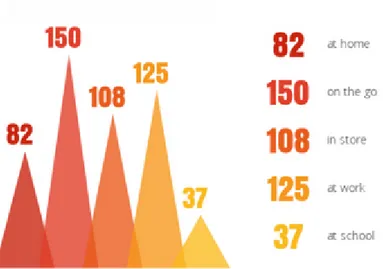
change of a property by age from a given database for data mining purposes [2] . . . 2 1.3 A visualization of homicides across Philadelphia since 2006 [3] . . 3 1.4 A visualization that shows the mobile searches for restaurants by

location of the customers based on data provided by Google. [4] . 3 1.5 A graph of the interacting characters in Christian Bible as a social

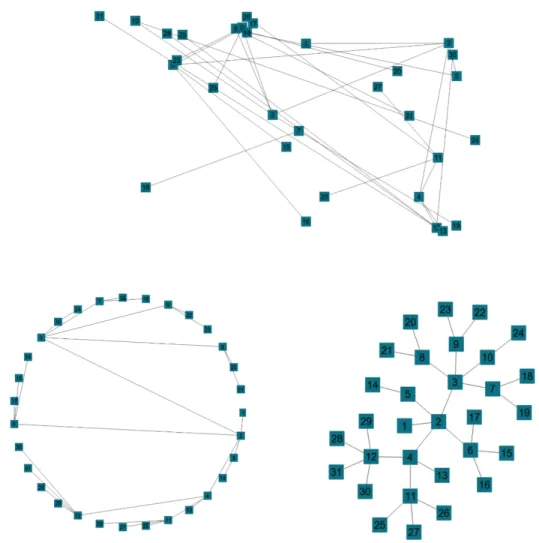
network [5] . . . 4 1.6 A random graph of 30 nodes drawn randomly, with circular layout

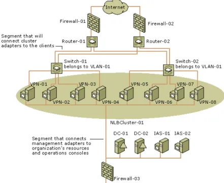
and CoSE layout respectively. [6] . . . 5 1.7 A cluster network graph that includes connectivity to clients, other

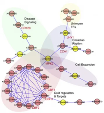
servers in an organization, and management and operations con-soles. Clustered VPN servers are shown in the shaded oval. [7] . . 6 1.8 A network of genes which belong to 5 distinct biological processes.

[8] . . . 7

LIST OF FIGURES ix

2.2 A simple compound graph [9] . . . 11

2.3 Two clustered graphs where one has no overlapping cluster (left) while the other does (right) [6] . . . 12

2.4 A friendship map from facebook data [10] . . . 12

2.5 ABB3 neighboring from PathwayCommons database visualized by Cytoscape [11] (left) and ChiBE [12] (right) . . . 13

2.6 A Watts and Strogatz network with a neighboring of four nodes and a random rewiring of 3 percent for each edge. . . 14

2.7 A scale free network of 60 nodes. . . 15

2.8 The spring analogy for graph layout [13] . . . 17

2.9 The magnitude of spring embedder forces [13] . . . 18

2.10 Part of a sample compound graph (left) and the corresponding physical model used by CoSE [14] . . . 20

2.11 The core structure of ChiLay in layout level with base layout classes are shown in detail. . . 23

2.12 The core structure of ChiLay in layout level with Force Directed Layout and CoSE Layout classes shown in detail. . . 24

2.13 A screenshot from ChiEd [6] . . . 26

2.14 i-Vis Sample Application that uses ChiLay remotely. [15] . . . 26

2.15 An Euler diagram that depicts the bacterial biogeography of the human digestive tract. [16] . . . 27

2.16 Class and zone naming conventions for the algorithm to visualize the overlapping sets. [17] . . . 28

LIST OF FIGURES x

2.17 An Euler diagram drawn using the algorithm to visualize the over-lapping sets. [17] . . . 29 2.18 Intersection graph for the example Euler diagram. . . 30 2.19 Overview of Simonetto’s drawing algorithm. (a) Initial

intersec-tion graph. (b) Intersecintersec-tion graph with layout. (c) The algorithm constructs a grid graph around the layout of the intersection graph. (d) Elements of the sets are added to the drawing, and the algo-rithm runs several iterations of a force directed layout algoalgo-rithm. [17] 30 2.20 Convex and non-convex polygons [18] . . . 31 2.21 Two polygons with separating axis in between them (left) and

Sep-arating Axis Theorem implementation is visualized for two sepa-rate polygons (right) [18] . . . 32 2.22 Separating Axis Theorem implementation is visualized for two

in-tersecting polygons [18] . . . 33

3.1 A cluster of two nodes bounded by a rectangle (left), an ellipse (middle) and a convex hull (right) where convex hull occupies the least space. . . 35 3.2 A cluster structure given as a Venn diagram (above) and its

cor-responding zone graph representation (below) . . . 36 3.3 A graph with overlapping clusters with six zones: 1, 2, 3, 1&2, 1&3

and 2&3 (left) and their corresponding zone polygons respectively: dark blue, light blue, yellow, purple, brown and black (right) . . . 37 3.4 A clustered graph with each cluster represented with a different

color (left) and the corresponding force directed model for the graph (right). Note that nodes 3 and 4 belong to two clusters. . . 38

LIST OF FIGURES xi

3.5 A graph with overlapping clusters to show different edge types in our layout algorithm. . . 40

4.1 A graph with overlapping clusters in which the nodes that are in-correctly placed inside the boundaries of other clusters are painted red. Nodes are labeled with the cluster IDs. . . 44 4.2 Running time comparisons of CoSE and Cluster Layout for

syn-thetic small world graphs up to 200 nodes . . . 44 4.3 Running time comparisons of CoSE and Cluster Layout for

syn-thetic scale free network graphs up to 500 nodes . . . 45 4.4 A plot that depicts the number of nodes that are placed inside the

boundaries of other clusters for CoSE and Cluster Layout using small world networks . . . 46 4.5 A plot that depicts the number of nodes that are placed inside the

boundaries of other clusters for CoSE and Cluster Layout using scale free networks . . . 47 4.6 Small world graphs of 40, 60 and 80 nodes clustered with OCG

and laid out with CoSE (left) and Cluster Layout (right). Nodes that are placed inside the boundaries of other clusters are painted red. . . 48 4.7 A real life graph of 242 nodes, based on gondola gene data laid out

with CoSE (left) and Cluster Layout (right) [19] . . . 49 4.8 A real life graph of 84 nodes, based on MST Transmission data,

laid out with CoSE (left) and Cluster Layout (right) [19] . . . 49 4.9 A real life graph of 186 nodes, based on Triticeae Glycolysis

LIST OF FIGURES xii

4.10 A real life graph of 34 nodes, based on Karate Club data, laid out with CoSE (left) and Cluster Layout (right) [21] . . . 50 4.11 A real life graph of 83 nodes, protein-protein interaction network

List of Tables

4.1 The number of nodes that are incorrectly placed inside the bound-aries of other clusters for CoSE and Cluster Layout for small world networks . . . 45

Chapter 1

Introduction

1.1

Motivation

Information visualization is a scientific field that aims to increase human under-standing on large data by visual representations. Visual elements help humans to perceive data in a more effective way. It is possible to find relationships, to discover similarities and to identify patterns in data with information visualiza-tion methods. Besides, visual elements help people to stay focused on a given subject. Instead of looking at a large textual table, a graph can explain much more about the nature of the information [23]. Maps, charts, graphs, dendograms can be given as examples of information visualization tools (Figure 1.1). Infor-mation visualization has applications in many areas such as scientific research, data mining (Figure 1.2), crime mapping (Figure 1.3), and marketing analysis (Figure 1.4).

As the graphical user interfaces evolved, the number of modern software that has visual features have increased. Visualization of relational data is usually achieved by graphs (Figure 1.5). Social, biological or computer networks can be given as examples for areas, where the graphs are used for visualization. Com-puter based visualization of relational information as graphs, makes it possible to make changes or queries over the data in an interactive way. Interactive graphs

Figure 1.1: Thermal maps of a dual-core AMD Athlon II 240 processor while running various CPU SPEC2006 [1]

Figure 1.2: A screenshot from the Data Surveyor software that depicts the change of a property by age from a given database for data mining purposes [2]

Figure 1.3: A visualization of homicides across Philadelphia since 2006 [3]

Figure 1.4: A visualization that shows the mobile searches for restaurants by location of the customers based on data provided by Google. [4]

also allow integration with other software systems via pre-defined standards such as SBML [24] or GraphML [25]. [9]

Figure 1.5: A graph of the interacting characters in Christian Bible as a social network [5]

Graph drawing is basically a pictorial view of a discrete set of objects (nodes) and a relation among these objects (edges). Nodes are usually drawn as circles, rectangles or dots, while edges are drawn as line segments or arcs. If the graph is directed, arrows are used for edge drawings. There are infinitely many ways to draw a single graph. [26]

Any of these infinite arrangements of nodes and edges is a layout. In visual-ization of complex data that is represented with graphs, it is important to present a good layout of the graph to the user to make the graph readable and under-standable. There are several criteria for good graph layout. The main aesthetics imply low number of edge crossings and overlapping nodes, and even distribution of nodes on the drawing area. Adjacent nodes should be close to each other and the size of the drawing area should be small in a good layout. [27] In Figure 1.6, there is a random tree with 30 nodes and 60 edges drawn with three different

layout approaches. The graph at the bottom is the most readable graph and it also satisfies the criteria of the scientific literature. The graph looks smaller in two upper drawings since the drawing area is large for random placement and circular layout.

Figure 1.6: A random graph of 30 nodes drawn randomly, with circular layout and CoSE layout respectively. [6]

One popular method for graph layout is using physical analogies [13]. This approach is known as the spring embedder algorithm. Spring embedders take the graph as a closed physical system where nodes are represented by positively charged particles and edges are represented by tiny springs in between these

particles. Particles repel each other while the springs keep the connected nodes closer to each other.

Relational information to be represented by graphs are usually clustered or hierarchically organized into groups in real life. Computer networks are usually clustered to provide fast and reliable services to clients Figure 1.7. An example to the hierarchical groups is organelles in a human cell. A cell is composed of cell wall and cytoplasm and the organelles that interact with each other within cytoplasm.

Figure 1.7: A cluster network graph that includes connectivity to clients, other servers in an organization, and management and operations consoles. Clustered VPN servers are shown in the shaded oval. [7]

Clustered graphs have been used in the past as a concept to represent more complex types of relationships with similar properties. The information is usually clustered and these clusters may overlap in the nature of biological, social and computer networks. There is a biological network with overlapping clusters in Figure 1.8. Genes are clustered according to the processes they are involved in this network. A gene that is involved in multiple processes resides in the intersection of these clusters. Although there is a huge effort to visualize relational information,

the literature is still lacking in taking clustered structures into account during automatic layout.

Figure 1.8: A network of genes which belong to 5 distinct biological processes. [8]

1.2

Contribution

In this thesis, we extended the compound spring embedder layout algorithm (CoSE) in order to visualize relational data with overlapping clusters. The spring embedder algorithm is modified with additional repulsion, spring forces and grav-itational forces so that

• When a convex hull is drawn around the nodes in a cluster, it only includes nodes that belong to this cluster.

• The clusters are separated in such a way that overlapping regions are close to the clusters that they belong to.

The algorithm was implemented as the Cluster Layout style of a layout and visualization library named Chisio. The algorithm was tested with small world graphs and some real life graphs. Preserving asymptotic running time complexity and the eye-pleasing properties of CoSE, the number of nodes that are placed inside the boundaries of other clusters are minimized with a reasonable overhead that is due to the calculation of new forces.

Chapter 2

Background and Related Work

2.1

Graphs

2.1.1

Basics and Definitions

A graph G = (V, E) is a pair of a vertex (node) set V and an edge set E. Two vertices u and v (u, v ∈ V ) are connected by an edge e = (u, v). Therefore, elements of E are subsets of V with two elements. Graph G is named as the owner graph for all edges and vertices. All vertices v ∈ V and edges e ∈ E are members of graph G. When an edge e = (u, v) is given, u and v are called neighbors or adjacent vertices or adjacent nodes. Also these two nodes are said to be incident to e. Two edges are said to be adjacent if they share a common node. [28]

Geometry of a graph may vary according to the application that it is going to be used in. Vertices can be represented by dots, circles, squares and many other shapes. Edges are usually denoted by straight or dashed lines or arcs between vertices. If the graph is directed, edges are represented by arrows. In order to store the geometry of a graph, the position of the nodes need to be kept at the least. The point that keeps the position of a node may be any reference point

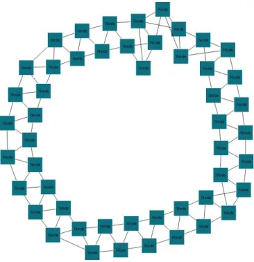
according to the implementation. A graph with 41 nodes is given in Figure 2.1.

Figure 2.1: A random graph with 41 nodes visualized by ChiEd software [6] A path (walk) in a graph is a sequence of nodes and edges that starts with a node and ends with a node such that adjacent nodes and edges in the sequence are neighbors. Number of edges in a path is the length of the path. A node can appear multiple times in a walk. Distance is the length of the shortest path between two nodes. In a graph, there can be more than one such path between two nodes. [29]

A compound graph is denoted by C = (V, E, F ) where V is nodes, E is edges and F is the inclusion graph [9]. The inclusion graph F = (V, F ) is a rooted tree to hold the hierarchical structure of the compound graph. In a compound graph E ∩ F = ∅, which means a node cannot be connected to its children or parent nodes. For the compound graph in Figure 2.2,

V = {a, b, c, d, e, f, g, h, i, j}

E = {{a, b}, {a, g}, {d, e}, {d, g}, {f, g}, {f, h}, {g, h}, {i, j}} F = {bc, bd, be, cf, cg, ch, ei, ej}

Figure 2.2: A simple compound graph [9]

The relational information to be visualized may be grouped into several cat-egories. When the entities in data have relations with each other and they have a set-like structure, it is convenient to visualize them with a clustered graph. In a clustered graph, nodes are assigned to clusters. If a node belongs to multiple clusters, then the graph is one with overlapping clusters. In Figure 2.3, the nodes are assigned to clusters and their cluster id numbers are written on them. Cluster bounds are drawn with polygons around the nodes. The graph on the right hand side is a graph with overlapping clusters since a node belongs to both clusters 1 and 3 and another node belongs to clusters 2 and 3.

2.1.2

Real Life Graphs, Small World Networks, and Scale

Free Networks

Real life graphs are those that represent real life relational information. For instance, a friendship map of a social network can be represented by such a graph (Figure 2.4). A biological network is another example of a real life graph (Figure 2.5).

Figure 2.3: Two clustered graphs where one has no overlapping cluster (left) while the other does (right) [6]

Figure 2.5: ABB3 neighboring from PathwayCommons database visualized by Cytoscape [11] (left) and ChiBE [12] (right)

A small world graph is a special type of mathematical network. In small world graphs, most of the nodes are not adjacent, but there are short paths to reach a node from another one. To be more precise, a graph is said to have the small-world property if the mean distance between pairs of nodes is small relative to the total number of nodes in the network. Usually, it is not desired that the distance between the nodes grow faster than logarithmic scale as the number of nodes is increased linearly. Given the distance as `,

` = O(logN )

Many networks in real life exhibit small world graph properties; therefore small world graphs are good for analysis of these networks and related algorithms. Road maps, food chains, neural networks, telephone call graphs, distributed systems, social influence networks, protein networks, transcriptional networks in biology are some examples to the concepts that show small world property. [30, 31] It is also useful for creating synthetic data for studies.

There are many proposed models for small world networks. Erdos-Renyi [32] proposed a model that exhibits a small average shortest path length. The clustering coefficient for Erdos-Renyi model is low. However, Watts and Stro-gatz realized that many real-world networks have a small average shortest path

length, along with a high clustering coefficient that tends to cluster the nodes to-gether. [33]. They proposed a new small-world graph model that provides these features.

Watts and Strogatz model is implemented in Boost graph library as a graph generation tool [34]. In this model, the graph is a ring graph, where each vertex is connected to its k nearest neighbors. Edges in the graph are randomly rewired to different vertices with a probability p (Figure 2.6). Here, p and k are determined by the user. Since nodes are always connected to the closest neighbors, small-world graphs have a high clustering coefficient, and the random rewiring makes it possible to have a small diameter.

Figure 2.6: A Watts and Strogatz network with a neighboring of four nodes and a random rewiring of 3 percent for each edge.

Another kind of synthetic network that is based on the real life information is scale free networks [35]. It is developed to mimic the characteristics of World Wide Web and genetic networks. In scale free networks, the probability P (k) that a vertex in the network interacts with k other vertices decays as a power law, following

P (k) ∼ k−γ, 2 ≤ γ ≤ 4

Scale free networks are generated by creating a node at each time step and connecting it to existing nodes according to the principal of “preferential at-tachment ”, where nodes with a higher degree have a higher probability of be-ing selected for attachment. At a timestep, the probability p of creating an edge between an existing node v and the newly added vertex is given to be p = deg(v)/|E|, where deg(v) is the degree of v and |E| is the number of edges in the network. Scale free networks are implemented in JUNG library to generate synthetic networks [36]. A scale-free network of 60 nodes is given in Figure 2.7.

2.2

Graph Drawing and Layout

As the amount of data grows, it is harder to represent it on the graph in such a way that it is understandable. Layout of the graphs often need to be automated to make use of the visual materials on analysis. There are several quality measures for graph drawings to evaluate their aesthetics and usability [26]. Neighboring nodes should be adjacent to provide the notion that the nodes are related. Nodes should not overlap and edge crossings should be minimized to increase readability. The drawing area should be small relative to the closest distance between any two vertices. The aspect ratio of the bounding box that surrounds the graph is also important.

There are several graph layout methods proposed for a good looking graph. Since every network has different characteristics, it is not possible to say that a method produces the best results for all graphs.

2.2.1

Force Directed Layout

Drawing on physical analogies is a widely used method for general graphs, de-signed free from any structural constraints. Here, the graph is considered as a physical system of interacting objects where the minimal energy state is consid-ered as an informative layout. Physical analogies are useful in the way that they are intuitive. Since it is an everyday experience for humans, it is easier to un-derstand and implement these algorithms. Besides, results are satisfactory since overlaps are avoided and edge crossings and drawing area are minimized [13].

Figure 2.8 shows an example, where the nodes are replaced with positively charged balls and the edges are substituted with springs in between. When this physical model is set free, positively charged balls will repel each other and springs will avoid the connected particles drift apart. Such a model can provide even distribution of nodes on the drawing area because of the repulsion forces and holds the adjacent nodes together. This model can be expressed either in terms of total energy of the system or in terms of forces. In this concept, force

directed layout is a popular method in graph drawing. In force directed layout, the system comes to the equilibrium state when all forces cancel each other. If this equilibrium state is not reached, the system is stopped after a predefined number of iterations.

Figure 2.8: The spring analogy for graph layout [13]

Given an undirected graph G = (V, E), let p = (pv)v∈V be a vector of vertex

positions pv = (xv, yv) in the plane. |pv− pu| being the Euclidian distance

be-tween positions pv and pu and −−→pupv being the unit vector pointing from pu to pv,

Eades [26] models a spring embedder where the repulsion and spring forces are defined as:

frep(pu, pv) =

crep

|pv− pu|2

fspring(pu, pv) = cspring· log

|pu − pv|

l · −−→pvpu

Here, crep and cspring are repulsion and spring constants respectively. l denotes

the spring length. Repulsion forces are applied between every pair of non-adjacent nodes. Instead of more realistic spring forces a logarithmic force is applied for the spring analogy for a weaker attraction to balance the repulsion forces. Spring forces are applied only between adjacent nodes since they are sufficient to keep the neighbors at a reasonable distance. In Figure 2.9 a qualitative impression of the forces a vertex u exerts on v is given, depending on the distance between them.

Figure 2.9: The magnitude of spring embedder forces [13]

In order to prevent the disconnected nodes to be placed apart from the rest of the graph, a weak gravitational force is also proposed, directed to the center of the drawing area.

The system should converge to a stable state after some iterations. Node positions that do not correspond to a system at equilibrium imply positive internal stress. Nodes are iteratively moved at time t according to a net force vector Fv(t), to relax the stressed system. Fv(t) is the sum of all spring and repulsion

forces that act on v. After computing Fv(t) for all nodes, each node is moved

σ times this vector. This constant σ is used to prevent nodes from changing its position too much to drift apart in a single iteration. After computing the forces iteratively, system comes to a stable state. A brief description of the spring embedder algorithm is given in Algorithm 1.

Algorithm 1 Brief description of the spring embedder algorithm [13] function SpringEmbedder(Graph G(V, E), Placement p = (pv)v∈V)

for t ← 1 to maximum number of iterations do for v ∈ V do

Fv(t) ←P_{u:{u,v} /}∈Efrep(pu, pv) +P_u:{u,v}∈Efspring(pu, pv)

end for for v ∈ V do pv ← pv + σ · Fv(t) end for end for end function

2.2.2

CoSE: Compound Spring Embedder

Compound Spring Embedder is a graph layout algorithm based on force-directed placement, which is extended to work also on compound graphs. In addition to that, CoSE can also handle non-uniform node sizes, inter-graph edges and clustered graph structures. [14]

CoSE extends the mechanical model proposed by Fruchterman and Reingold. It simulates the mechanical system where nodes and edges are modeled by posi-tively charged particles and springs respecposi-tively.

A compound node is treated as a single object in CoSE [14]. It is modeled like an elastic cart. In a compound node, compound structure is kept as a child graph. A compound node has its own center. It can move in orthogonal directions. Its

size can vary depending on the bounding box of its child graph. (Figure 2.10) Repulsive forces are calculated per graph. In other words, there is no interaction between a node in child graph and a node in parent graph for the sake of simplicity and efficiency. Ideal edge lengths of intra-graph edges are predefined per layout and are equal to each other. Ideal edge lengths of inter-graph edges are calculated with proportion to the compound depth.

Figure 2.10: Part of a sample compound graph (left) and the corresponding physical model used by CoSE [14]

Many layout algorithms assume nodes as points or uniform sized shapes mak-ing it easier to calculate distances between the nodes. CoSE supports different node sizes by calculating the distance between the nodes. This distance is the clipping points of the line that passes through the centers of the nodes. Although it is costly, it is needed for compound node support.

CoSE starts with initialization of the spring and repulsion constants. At first nodes are placed randomly. After the initialization, attraction, repulsion and gravitational forces are applied iteratively to the system. Temperature of the system is cooled down periodically to allow the system to stop at a stable state. The system stops after total movement of the nodes is less than a threshold value.

The attraction forces are calculated for each edge while the repulsion forces are calculated for every node pair. The repulsion force between two nodes is not calculated if the distance between them is higher than some threshold value. Since it is still needed to calculate the distances, the complexity of one iteration of CoSE algorithm is O(|E| + |V2|).

Later, Kara¸celik improved the runtime of CoSE algorithm by using FR-Grid Variant method, multi level scaling and GPU parallelism [9].

2.2.3

ChiLay: Chisio Layout

Chisio Layout (abbreviated as ChiLay) is an open source graph layout library [37]. It can be used by interactive graph editing tools to layout different types of graphs such as simple, compound, clustered or hierarchically structured graphs. It can be used locally or remotely. ChiLay has some popular layout algorithms already implemented such as Force Directed Layout, Spring Layout, Sugiyama Layout, and AVSDF Layout. Algorithms developed by Bilkent University Information Visualization Group are also included in ChiLay. Those algorithms are CiSE, CoSE, Cluster Layout, and SBGN Layout.

There are two separate levels to point out the layout and view related infor-mation of a layout (l-level) and view (v-level). Each l-level graph object is related to a v-level object. The graph objects hold pointers to the node and edge objects along with other graph data. A node object has graph property too. However, this is not a pointer to the root graph. It is for compound nodes to hold the sub-graph information such as inner nodes and edges that the node represents. ChiLay has an object oriented design that is modular and extendible. [38]

Data structures that we used through the implementation of the algorithm follow the software architecture of ChiLay Library. For clearity, the core structure in layout level is given in Figure 2.11 and 2.12. LGraphObject is the base class for all objects in the layout level such as LGraph, LNode and LEdge. LGraphObject holds the reference for view-level objects with vGraphObject property. Each node

has a reference to his owner graph since compound nodes have their own graphs to hold the other nodes within. Edges have source and target pointers. Also all nodes have their incident edges listed. LGraphManager has the complete graph topology. There is the compound graph structure in LGraphManager. It also maintains the inter-graph edges.

Figure 2.11: The core structure of Chi La y in la y ou t lev el with base la y out classes are sho wn in deta il.

Figure 2.12: The core structure of ChiLa y in la y out lev el with F orce Directed La y out and CoSE La y out classes sho wn in detail.

Layout class is the base class for all layout algorithms that are implemented in Chisio according to the structure in LGraphManager. Both layout and graph manager classes hold references to each other. Each l-level node and edge is associated with a v-level node and edge, respectively. Layout class makes the necessary callbacks to update methods in the view level. The changes in layout level are reflected to the view level objects via updates after the layout process is done. The manipulations on the view level objects are reflected to the layout level objects since view level objects implement the Updateable interface. Chisio gives the users the opportunity to customize layout algorithms. Also pre and post layout operations may be performed by customizing the respective methods in Layout class. In addition to these customizations, new layout styles can be implemented by extending Layout class.

Chisio Layout can be used both locally, as part of an application, or remotely, for instance by a web application. ChiEd: Chisio Editor [6] is a graph visualiza-tion applicavisualiza-tion in Java for creating, editing and layout of compound or clustered graphs as well as flat graphs. It uses the ChiLay component for layout services. All of the layout algorithms implemented in ChiLay can be used to visualize graphs in ChiEd. 2.13. Users also can deploy Chisio to a server to benefit from the remote layout services. In order to use Chisio Layout as a remote service properly, the graph geometry should be saved in XML format that conforms to the schema given in Chisio Programmers Guide. After that, the saved XML con-tent must be sent to the server via an HTTP request. Server takes the request, performs the layout operation and sends back an XML content that has the graph geometry after layout process. In Figure 2.14, there is a web application that uses ChiLay’s layout services remotely.

2.3

Automatic

Visualization

of

Overlapping

Sets

Visualization of hierarchical information is usually described by sets. Many tech-niques are proposed for visualization of sets. These techtech-niques include tree maps

Figure 2.13: A screenshot from ChiEd [6]

and directed acyclic graphs. However, these methods result in a visualization that is too complex and hard to analyze. Euler diagrams are suitable matches for visualizing overlapping sets.

Euler diagrams are graphical representations that show sets and their inter-sections. In an Euler diagram, a set is a region bounded by a closed curve or polygon. Set intersections are shown by overlaps of these bounded regions. (Fig-ure 2.15) Although Euler diagrams are used in visualizing sets for hundreds of years, the problem of automatic generation of these diagrams is a relatively new topic.

Figure 2.15: An Euler diagram that depicts the bacterial biogeography of the human digestive tract. [16]

Simonetto et al. proposed an algorithm for drawing Euler diagrams auto-matically [17]. They proposed the concepts of zones, classes and an intersection graph. In order to provide a better understanding of the study, some terminology will be introduced.

Given a subset S of the sets in the Euler diagram, a zone is a region in the diagram where all and only the elements of S intersect. A zone is also the subset of elements contained by region.

Classes are the sets illustrated in the drawing of the Euler diagram.

In Figure 2.16, classes are represented by capital letters and zones are repre-sented by lowercase letters and their combinations. The listing of the classes is given as input to the algorithm in set notation.

Figure 2.16: Class and zone naming conventions for the algorithm to visualize the overlapping sets. [17]

For instance, the input for the Euler diagram in Figure 2.17 is as follows. Monuments = {Eiffel Tower, Colesseum, Taj Mahal, Big Ben, Great Wall of China, Statue of Liberty}

France = {Wine, Baugette, Eiffel Tower} Italy = {Colesseum, Pasta, Pizza}

In Figure 2.17, the red colored set contains world monuments, the green col-ored set contains things that are typically Italian, and the blue colcol-ored set con-tains things that are typically French. The red colored set shares the element “Colosseum” with the green colored set and the element “Eiffel Tower” with the blue colored set as demonstrated through overlaps of the regions.

The algorithm firstly forms an intersection graph from the input sets. Algo-rithm basically works as follows:

• Construct a planar drawing of the intersection graph.

• Build a grid graph around the intersection graph, mapping nodes of inter-section graph to zones.

Figure 2.17: An Euler diagram drawn using the algorithm to visualize the over-lapping sets. [17]

• Insert the elements into their zones and apply a force directed algorithm to obtain a good placement.

• Select colors and textures for the classes and use Bezier curves to draw the class boundaries.

Each node in the intersection graph is a zone. There is an edge between two nodes if their related zones are adjacent. In Figure 2.18, the intersection graph for the Euler diagram above is given. The drawing of the intersection graph should be planar and should minimize the number of edge crossings to avoid undesired overlaps in the visualization of sets. A force directed layout algorithm is applied to the intersection graph to achieve this. Applying force directed algorithm also paves the way for the faster convergence of the overall algorithm.

Mapping between the intersection graph and the regions in the Euler diagram is done through another graph named grid graph (Figure 2.19). The grid graph draws the rough boundaries of the Euler diagram by enclosing each node and edge of the intersection graph. The boundaries are drawn in non overlapping regions of the plane. To construct the grid graph, a set of non-overlapping circles are computed. These circles are placed around each node such that the centers of

Figure 2.18: Intersection graph for the example Euler diagram.

the circles are the positions of the nodes of the intersection graph. These circles are small enough to avoid overlaps.

Figure 2.19: Overview of Simonetto’s drawing algorithm. (a) Initial intersection graph. (b) Intersection graph with layout. (c) The algorithm constructs a grid graph around the layout of the intersection graph. (d) Elements of the sets are added to the drawing, and the algorithm runs several iterations of a force directed layout algorithm. [17]

After that, node and edge regions are defined in the grid graph. Elements are placed inside these circles according to the sets they belong to. Then, the drawing of the grid graph is refined by a force directed layout algorithm.

Lastly, the final set boundaries are drawn with Bezier curves and each set is refined by a distinct color.

2.4

Polygons and Separating Axis Theorem

A polygon is a closed region of the plane enclosed by a simple cycle of straight line segments. A simple cycle means that nonadjacent segments do not intersect and two adjacent segments intersect only at their common end point [39]. Tri-angles, rectTri-angles, and octagons are all examples of polygons. A convex hull is a list of ordered points in software systems. They are implemented as polygons. The polygonal chain constructed from this ordered list of points determines the boundary of the polygon. A convex hull reflects a convex polygon, that is, for any pair of points p, q ∈ S the line segment pq is completely contained in S where S is a polygon [40]. See Figure 2.20 for the examples of convex and non-convex polygons.

Figure 2.20: Convex and non-convex polygons [18]

In order to detect if two convex polygons intersect, Separating Axis Theorem is used. Let P and Q be two convex polygons and l be a line on the same plane. Separating Axis Theorem states that if a line l divides the plane into two subsets S1 and S2 such that P ∈ S1 and Q ∈ S2, then the P and Q are not intersecting.

This theorem is highly applicable to software systems, providing a faster so-lution than pixel based algorithms. The idea is to find a line in between two polygons to prove that they are not intersecting. There are infinitely many lines on a plane so in order to obtain a solution, linear projections of the polygons are taken with respect to the normal vectors to the polygon edges. An outline of the algorithm is given in Algorithm 2.

Algorithm 2 Algorithm to check if two polygons are overlapping function ArePolygonsIntersecting(Polygon A, Polygon B)

for all edges in A and B do

find the axis perpendicular to the current edge. project both polygons on that axis.

if projections overlap then return false

end if end for return true end function

axes perpendicular to the edges are calculated, it is possible to find a minimal translation vector to separate the polygons(Figure 2.22). If one of these polygons are pushed apart by this vector, polygons do not intersect.

Figure 2.21: Two polygons with separating axis in between them (left) and Sep-arating Axis Theorem implementation is visualized for two separate polygons (right) [18]

2.5

Generating Overlapping Clusters

Real life data is usually clustered and the clusters are overlapping in many cases. One example to this is multifunctional proteins. Protein-protein interaction (PPI)

Figure 2.22: Separating Axis Theorem implementation is visualized for two in-tersecting polygons [18]

networks show the modularity of processes in a cell and makes the protein func-tions more understandable. In PPI networks, nodes are proteins and edges are direct physical interactions. PPI networks are usually clustered as functional modules. Here, multifunctional proteins reside in more than one cluster making the network a graph with overlapping clusters.

Becker et al. presented a clustering method named OCG (Overlapping Cluster Generator) [41]. The algorithm decomposes a network into overlapping clusters. The algorithm is verified by PPI networks. The multifunctional proteins appeared at the intersection of clusters.

Chapter 3

Overlapping Cluster Layout

Algorithm

Simonetto et al. proposed an algorithm to visualize overlapping sets. We decided to visualize graphs with overlapping clusters, inspired by their work on sets. In the graphs used for this study, a node can belong to multiple clusters. Although this problem is encountered in many real life cases, there is no other study on this in the literature.

There is no standard representation for the visualization of clusters or sets. The previous ones mostly use circular visualization assigning different shapes or colors to cluster elements. The approach varies depending on the specific domains that the graphs are used in.

More important point is that no previous method suggests a way to visualize graphs with overlapping clusters. Using simpler geometric shapes such as ellipses, circles or rectangles to bound the clusters is problematic in visualizing overlapping clusters. The main reason is that they waste too much space on the drawing area. When there are overlaps between the clusters these empty spaces affect the total area and the graph readability even worse. A good example is Venn diagrams. Venn diagrams usually depict the sets as circular shapes and the fact is it is impossible to draw a Venn diagram to visualize all intersections of 4 or more

sets [42].

Therefore it is more convenient to use polygons obtained by the convex hull method as a bounding shape for clusters to keep the drawing area of each cluster as small as possible to be able to save space for the intersecting regions (Fig-ure 3.1).

Figure 3.1: A cluster of two nodes bounded by a rectangle (left), an ellipse (middle) and a convex hull (right) where convex hull occupies the least space.

3.1

Zone Graph

In our modification on Simonetto’s algorithm, first we build a zone graph for the clustered graph to be drawn. This is an upper level graph such that we call it to be virtual, since it is not contained in the original graph data. This virtual graph corresponds to the intersection graph in Simonetto’s study on overlapping sets. In this virtual zone graph, nodes correspond to zones, which are cluster intersections and the non-intersecting parts of a cluster. In a zone graph, edges are placed between the non-intersecting zones and their corresponding cluster intersection zones. Since the zone graph is undirected, the order of the lowercase letters does not matter. In Figure 3.2, there are three clusters, drawn as a Venn diagram. On this figure, lowercase lettered areas are zones, and uppercase letters represent clusters. A single lowercase letter represents a non-intersecting zone while multiple lowercase letters stand for an intersection zone. The corresponding zone graph for such a cluster structure is also given in Figure 3.2. Edges and nodes in the zone graph are called zone edges and zone nodes, respectively. When we use

the term graph, we will be referring to the actual graph (the clustered, possibly having overlapping clusters). For the virtual graph that represents zones, on the other hand, we use the term zone graph.

Figure 3.2: A cluster structure given as a Venn diagram (above) and its corre-sponding zone graph representation (below)

The shape that we choose to use for zones is crucial for our approach to be successful. Not only the shapes of the zones directly affect the quality of our layouts, but also they are crucial for the running time of the algorithm. As explained formerly, we use convex polygons as zone shapes (Figure 3.3). A zone polygon covers all nodes that reside in the zone. Notice here that nodes themselves are allowed to have varying dimensions, represented with rectangles. Convex polygon operations are less costly to calculate when they are compared to the concave polygons. Convex polygons provide a better packing than rectangles and circles, so the drawing area is kept small.

3.2

Modified Spring Embedder

After building the zone graph as explained, the layout for this graph is performed together with the whole graph with a force directed approach iteratively. We build our algorithm on CoSE layout. Zones are considered as positively charged

Figure 3.3: A graph with overlapping clusters with six zones: 1, 2, 3, 1&2, 1&3 and 2&3 (left) and their corresponding zone polygons respectively: dark blue, light blue, yellow, purple, brown and black (right)

particles and the edges between the zones act as the springs (Figure 3.4). Posi-tively charged zones repel each other and springs keep the related non-intersecting zones and intersection zones close to each other.

The forces for the zone graph are calculated in each iteration like the tradi-tional spring embedder forces. The forces for the zone graph are added to the related nodes in the actual graph in each iteration. After moving the nodes in the graph according to the total force, the positions and shapes of the zone polygons are recalculated.

The algorithm Cluster Layout is based on CoSE algorithm. We propose ad-ditional forces to the traad-ditional spring and repulsion forces.

Calculation of the repulsion forces between the zone nodes is built over the method that calculates the repulsion forces in CoSE. After the forces are calcu-lated for the actual graph, repulsion forces are calcucalcu-lated for the zone nodes with the method given in Algorithm 3. Here, Z and |Z| denotes the zones and the number of zones, respectively. Similarly N is the set of nodes. n.zone is the zone

Figure 3.4: A clustered graph with each cluster represented with a different color (left) and the corresponding force directed model for the graph (right). Note that nodes 3 and 4 belong to two clusters.

node that n resides in. z denotes a zone node such that z ∈ Z.

Algorithm 3 Brief description of the method to calculate the repulsion forces for zone nodes

function CalculateZoneGraphRepulsionForces(Z) for i ← 0 to |Z| − 1 do for j ← i + 1 to |Z| do CalculateRepulsionForce(zi, zj) end for end for for all n ∈ N do

n.frep ← n.frep+ n.zone.frep

end for end function

The repulsion forces for the zone nodes are calculated the same way as CoSE nodes. The method to calculate the repulsion force between each pair of nodes is briefly explained in Algorithm 4. The clipping points are the intersection points of the polygons and the line segment between the centeroids of the polygons. If zones overlap, the repulsion force becomes equal to the amount of overlap in x and y directions. If they do not overlap, the distance between the zones are calculated along with the clipping points of the zones and the force is inversely proportional to the square of the distance between them. Also, there is a repulsion constant

to control the amount of repulsion.

Algorithm 4 Brief description of the repulsion force calculation between two nodes

function CalculateRepulsionForce(ni, nj)

if ni.CalculateOverlap(nj,overlap) then

ni.frep ← overlap

nj.frep ← −overlap

else

Calculate distance between ni and nj

frep ← REP U LSION CON ST AN T_distance

end if return frep

end function

The CalculateOverlap method is executed for each node pair depending on the geometric shape of the nodes. For zone nodes, this method adopts the separating axis theorem implementation. The method returns a Boolean value to identify if there is an overlap along with the smallest translation vector as the smallest vector to separate these two zones. The CalculateOverlap method for zone nodes is briefly explained in Algorithm 5.

Algorithm 5 Brief description of the method of a zone node zi that detects if

there is an overlap with a zone node zj and returns the overlap amount

function CalculateOverlap(zj, overlap)

overlap ← ConvexPolygonOverlap(ni.polygon, nj.polygon)

if overlap 6= 0 then return true else return false end if end function

The ConvexPolygonOverlap method calculates the minimum translation vec-tor according to separating axis theorem. Its implementation is given in Ap-pendix A.

The spring forces for the zone graph are calculated in a very similar way to the repulsion forces. The CalculateSpringForces method is modified to calculate the spring forces in zone graph caused by the zone edges.

The spring lengths are crucial to keep the neighboring nodes at a safe distance. Ideal edge lengths for the edges are determined for each edge at the beginning of layout to be used during the layout process. Since we want to keep the nodes that reside in the same cluster close to each other, we propose different edge lengths according to the cluster connectivity. We have three types of edges in a graph with overlapping clusters named intra-zone, zone-neighbor, and inter-zone edges in increasing lengths. An edge is intra-zone if it connects two nodes of the same zone, zone-neighbor if it connects two nodes of the same cluster but different zones, and inter-zone if it connects two nodes of different clusters (Figure 3.5).

Figure 3.5: A graph with overlapping clusters to show different edge types in our layout algorithm.

With Ez being the list of zone edges, ez ∈ Ez, ez.target and ez.source being

the target and source zone nodes of ez, respectively, the spring force calculation

method for the zone graph is explained in Algorithm 6.

Apart from the gravitation to the center of the drawing area, an additional gravitational force is applied to each node. This new gravitational force points to the center of the zone polygon that the node belongs to. This provides compact-ness for the graph. The calculation method is explained in Algorithm 7 where Z is the set of zones, N is the set of nodes and g is the local gravitation constant.

The overall modified spring embedder method is given in Algorithm 8. While updating the bounds for the graph, the zone polygons are also updated after each

Algorithm 6 Brief description of the method to calculate the spring forces for the zone graph

function CalculateZoneGraphSpringForces() for all ez ∈ Ez do

CalculateSpringForce(ez.target, ez.source)

end for

Apply calculated forces to the zone members for all n ∈ N do

n.fspring ← n.fspring+ n.zone.fspring

end for end function

Algorithm 7 Brief description of the method to calculate the gravitational forces for the zone graph

function CalculateZoneGraphGravitationalForces() for all z ∈ Z do

for all n ∈ z do

distanceX ← n.x − z.x distanceY ← n.x − z.y

n.gravitationF orceX ← −g ∗ distanceX n.gravitationF orceY ← −g ∗ distanceY end for

end for end function

iteration.

Algorithm 8 Brief description of the method to calculate the gravitational forces for the zone graph

function SpringEmbedder()

for t ← 1 to maximum number of iterations do Update Bounds

Calculate Spring Forces

Calculate Zone Graph Spring Forces Calculate Repulsion Forces

Calculate Zone Graph Repulsion Forces Calculate Gravitational Forces

Calculate Zone Graph Gravitational Forces Move Nodes

end for end function

Chapter 4

Experimental Results

In order to test the execution time and quality of layouts produced by Clus-ter Layout, a set of real life graphs, synthetic small world network graphs, and synthetic scale free network graphs are used [34].

Some of these real life graphs were obtained from the literature and were readily clustered by the authors, considering real properties of the entities repre-sented by the nodes. The synthetic small world graphs, on the other hand, were generated using Small World Generator of Boost Graph Library [34]. For these synthetic graphs and some of the real life graphs that were not clustered, we used Becker’s Overlapping Cluster Generator [41] to obtain overlapping clusters.

For performance comparisons, tests are run with the same graphs and the same system configuration of a Java VM running on 2.13 GHz Intel(R) Core(TM) i3 CPU and 3 GB of installed memory. The results are compared to CoSE algorithm for running time. The main quality criterion has been based on the number of nodes that were incorrectly placed inside the boundaries of clusters that a particular node does not belong to (Figure 4.1).

The running time comparison of Cluster Layout and CoSE for the Watts and Strogatz small world network graphs is given in Figure 4.2. The running time

Figure 4.1: A graph with overlapping clusters in which the nodes that are incor-rectly placed inside the boundaries of other clusters are painted red. Nodes are labeled with the cluster IDs.

comparison for scale free networks is given in Figure 4.3. In these tests, we an-alyzed the change in running time with respect to number of nodes as well as number of clusters. The same graphs are clustered with OCG with changing the maximum cluster size from 15 nodes to 40 nodes. The results are the average run-ning time of 10 layouts for each graph in miliseconds. Additional forces increase the running time two to three times.

Figure 4.2: Running time comparisons of CoSE and Cluster Layout for synthetic small world graphs up to 200 nodes

The number of nodes that are placed inside the boundaries of other clusters for CoSE and Cluster Layout is given in Table 4.1. Again the numbers are

Figure 4.3: Running time comparisons of CoSE and Cluster Layout for synthetic scale free network graphs up to 500 nodes

40 60 80 100 120 140 160 CoSE 1.1 3.3 11.2 30.2 48.7 60.9 84.7 Cluster 0.1 1.5 3.6 24.8 29.9 59.9 81.7

Table 4.1: The number of nodes that are incorrectly placed inside the boundaries of other clusters for CoSE and Cluster Layout for small world networks

the averages of 10 layouts for each graph. With our Cluster Layout algorithm, number of misplaced nodes are greatly reduced especially for small to medium sized graphs. The plots to compare the number of misplaced nodes for small world networks and scale free networks are also given in Figure 4.4 and Figure 4.5. Some layout examples of the small world graphs are given in Figure 4.6.

Figure 4.4: A plot that depicts the number of nodes that are placed inside the boundaries of other clusters for CoSE and Cluster Layout using small world net-works

We also tested Cluster Layout algorithm with the clustered real life graphs from the literature. In Figures 4.7, 4.8, 4.9, 4.10, and 4.11, there are some example layouts of these real life graphs with CoSE and Cluster Layout.

Despite the increase in the running time and the total drawing area, the num-ber of nodes that are placed inside the boundaries of other clusters is minimized, especially for small to medium sized graphs. The algorithm gives excellent results for small world graphs up to 120 nodes due to the nature of those networks. In small world networks, the average distance between the nodes is small and the graph topology is closed such that after layout, the intersection zones reside on the middle of the drawing area, which are surrounded by a circle of non-intersecting zones. The dense structure causes to nodes to get closer to each other, therefore there are many misplaced nodes in the middle of the drawing area. Another rea-son is that, apart from CoSE, new forces cause the overall system to converge in

Figure 4.5: A plot that depicts the number of nodes that are placed inside the boundaries of other clusters for CoSE and Cluster Layout using scale free networks later iterations. Algorithm always give better results for scale free networks. The number of misplaced nodes is minimized when it is compared to CoSE. For real graphs, algorithm gives visually good results up to 300 nodes. Since the force directed layout is normally expected to yield nice layouts for up to 100 nodes [13], the results are satisfactory for the graph drawing criteria through a visual inspec-tion. Although there is an increase in running time due to the calculation of new types of forces, the algorithm is still suitable for interactive use, at least for graphs of small to medium sizes.

Figure 4.6: Small world graphs of 40, 60 and 80 nodes clustered with OCG and laid out with CoSE (left) and Cluster Layout (right). Nodes that are placed inside the boundaries of other clusters are painted red.

Figure 4.7: A real life graph of 242 nodes, based on gondola gene data laid out with CoSE (left) and Cluster Layout (right) [19]

Figure 4.8: A real life graph of 84 nodes, based on MST Transmission data, laid out with CoSE (left) and Cluster Layout (right) [19]

Figure 4.9: A real life graph of 186 nodes, based on Triticeae Glycolysis Chloro-plast, laid out with CoSE (left) and Cluster Layout (right) [20]

Figure 4.10: A real life graph of 34 nodes, based on Karate Club data, laid out with CoSE (left) and Cluster Layout (right) [21]

Figure 4.11: A real life graph of 83 nodes, protein-protein interaction network of yeast, laid out with CoSE (left) and Cluster Layout (right) [22]

Chapter 5

Conclusion

In this study, we propose an algorithm to visualize graphs with overlapping clus-ters. Inspired by the Simonetto’s work on visualizing overlapping sets [17], we divide the clustered graph into sections called zones. Zones are formed consid-ering the intersection of the clusters. Assigning an edge between the zones that make up a cluster, we define a virtual zone graph for the divided sections. Our algorithm is built on Compound Spring Embedder (CoSE) algorithm calculating the newly introduced forces for this virtual graph, while calculating forces for the other nodes in the traditional way. This way, we manage to show the nodes in overlapping regions in between the cluster regions that they are shared. The number of nodes that reside in the boundaries of other clusters is decreased dras-tically for small to medium sized graphs at the cost of an increase in the total drawing area and running time by a constant factor.

We tested the algorithm with real life graphs, synthetic scale free network graphs, and synthetic small world graphs. We get satisfactory results in real life graphs up to about 300 nodes. The number of misplaced nodes is minimized for scale free networks. Because small world networks have more cycles, as the number of nodes increase the new forces fail to separate the clusters. However, the results are again satisfactory up to around 120 nodes.

5.1

Parameter Tuning

Parameters like spring constant, repulsion constant, and cooling factor should be considered to be tuned since they change the quality and the running time of the layout directly.

Higher spring constants caused the graph to come to an equilibrium state slower. Higher repulsion constants mean larger drawing area, but visually better results.

In this work, modifying the constants at each step of development, we slightly increased the repulsion constant. We also proposed new edge types and fine tuning on their desired lengths is done experimentally to have the best possible visual results.

5.2

Future Work

A disadvantage of the algorithm is the running time overhead due to the new forces. The effort to lower the running time may be achieved by using GPU parallelism for polygon calculations. This may be useful especially for larger graphs where there are many zones.

At the time this work was done, there was a small number of work on clustering algorithms that allows overlapping clusters. As the number of work on this area increases, new tests can be applied to fine tune the algorithm with respect to the clustering caused by the new clusterers.

5.3

Availability

All of the improvements that are mentioned in this thesis are implemented under overlapping clusters branch of Chisio Layout (ChiLay) project. It is stored in a

Bibliography

[1] “Scalable computing systems laboratory (scale).” http://scale.engin. brown.edu/tools/, Accessed in June 2014.

[2] “Data mining.” https://www.siggraph.org/education/materials/ HyperVis/applicat/data_mining/data_mining.html, Accessed in June 2014.

[3] “5 ways of visualizing crime in philly.” http://www.citylab.com/crime/ 2013/02/5-ways-visualizing-crime-philadelphia/4641/, Accessed in June 2014.

[4] “Google just put the market research biz on notice.” http://gigaom.com/ 2013/07/10/google-just-put-the-market-research-biz-on-notice/, Accessed in June 2014.

[5] “Mapping new testament social networks.” http://www.crossway.org/ blog/2007/01/mapping-nt-social-networks/, Accessed in June 2014. [6] “Chied: Chisio editor.” http://cs.bilkent.edu.tr/~ivis/chied.html,

Accessed in June 2014.

[7] “Selecting the number of network adapters in each cluster host.” http:// technet.microsoft.com/en-us/library/cc738475(v=ws.10).aspx, Ac-cessed in July 2014.

[8] “Msu-doe plant research laboratory.” http://www.prl.msu.edu/faculty/ chen_jin, Accessed in July 2014.

[9] A. Karacelik, “An improved spring embedder layout algorithm for compound graphs,” Master’s thesis, Bilkent University, 2012.

[10] “Visualizing your facebook network of friends.” http://www.messersmith.name/wordpress/2009/10/12/

visualizing-your-facebook-network-of-friends/, Accessed in August 2014.

[11] “Cytoscape: An open source platform for complex network analysis and visualization.” http://www.cytoscape.org/, Accessed in June 2014. [12] “Chibe: Chisio biopax editor.” https://code.google.com/p/chibe/,

Ac-cessed in June 2014.

[13] U. Brandes, “Drawing on physical analogies,” in Drawing Graphs (M. Kauf-mann and D. Wagner, eds.), vol. 2025 of Lecture Notes in Computer Science, pp. 71–86, Springer Berlin Heidelberg, 2001.

[14] U. Dogrusoz, E. Giral, A. Cetintas, A. Civril, and E. Demir, “A layout algorithm for undirected compound graphs,” Information Sciences, vol. 179, no. 7, pp. 980 – 994, 2009.

[15] “i-vis layout demo.” _{http://www.cs.bilkent.edu.tr/~ivis/layout/} demo/lw1x.html, Accessed in June 2014.

[16] e. a. Jennifer C. Stearns, Michael D. J. Lynch, “Bacterial biogeography of the human digestive tract,” 2011.

[17] P. Simonetto, D. Auber, and D. Archambault, “Fully automatic visualisation of overlapping sets,” in Proceedings of the 11th Eurographics / IEEE -VGTC Conference on Visualization, EuroVis’09, (Aire-la-Ville, Switzerland, Switzerland), pp. 967–974, Eurographics Association, 2009.

[18] “Sat: Separating axis theorem.” http://www.codezealot.org/archives/ 55, Accessed in June 2014.

[19] “Social network generation.” http://www.infovis-wiki.net/index.php? title=Social_Network_Generation, Accessed in July 2014.

[20] “Data linkage graphs.” http://pgrc.ipk-gatersleben.de/dlg/, Accessed in July 2014.

[21] “Clique graphs and overlapping communities.” http://ej.iop.org/ images/1742-5468/2010/12/P12037/Full/7734302.jpg, Accessed in July 2014.

[22] “Cfinder clusters and communities: overlapping dense groups in networks.” http://www.cfinder.org, Accessed in July 2014.

[23] B. Shneiderman and B. B. Bederson, The Craft of Information Visualiza-tion: Readings and Reflections. San Francisco, CA, USA: Morgan Kaufmann Publishers Inc., 2003.

[24] “Systems biology markup language.” http://sbml.org/Main_Page, Ac-cessed in June 2014.

[25] “The graphml file format.” http://graphml.graphdrawing.org, Accessed in June 2014.

[26] P. Eades and R. Tamassia, “Algorithms for drawing graphs: An annotated bibliography,” tech. rep., Providence, RI, USA, 1988.

[27] T. M. J. Fruchterman and E. M. Reingold, “Graph drawing by force-directed placement,” Softw. Pract. Exper., vol. 21, pp. 1129–1164, Nov. 1991.

[28] R. Diestel, Graph Theory (Graduate Texts in Mathematics). Springer, Au-gust 2005.

[29] M. E. J. Newman, “The structure and function of complex networks,” SIAM REVIEW, vol. 45, pp. 167–256, 2003.

[30] R. Cohen and S. Havlin, “Scale-Free Networks Are Ultrasmall,” Phys. Rev. Lett., vol. 90, p. 058701, 2003.

[31] P. Bork, L. Jensen, C. von Mering, A. Ramani, I. Lee, and E. Marcotte, “Protein interaction networks from yeast to human,” Current Opinion in Structural Biology, vol. 14, no. 3, pp. 292–9, 2004.