Exciton induced directed motion of unconstrained atoms in an ultracold gas

(1)

Journal of Physics B: Atomic, Molecular and Optical Physics

PAPER

Exciton induced directed motion of unconstrained

atoms in an ultracold gas

To cite this article: K Leonhardt et al 2017 J. Phys. B: At. Mol. Opt. Phys. 50 054001

View the article online for updates and enhancements.

-Recent citations

Rydberg aggregates S Wüster and J-M Rost

-Quantum dynamics of long-range interacting systems using the positive- P and gauge- P representations S. Wüster et al

(2)

Exciton induced directed motion of

unconstrained atoms in an ultracold gas

K Leonhardt

1

, S Wüster

1,2,3

and J M Rost

1

Max Planck Institute for the Physics of Complex Systems, Nöthnitzer Strasse 38, D-01187 Dresden, Germany

2

Department of Physics, Bilkent University, 06800 Çankaya, Ankara, Turkey

3_{Department of Physics, Indian Institute of Science Education and Research, Bhopal, Madhya Pradesh 462}

023, India

E-mail:karlo@pks.mpg.de

Received 3 August 2016, revised 21 December 2016 Accepted for publication 4 January 2017

Published 14 February 2017 Abstract

We demonstrate that through localised Rydberg excitation in a three-dimensional cold atom cloud atomic motion can be rendered directed and nearly confined to a plane, without spatial constraints for the motion of individual atoms. This enables creation and observation of non-adiabatic electronic Rydberg dynamics in atoms accelerated by dipole–dipole interactions under natural conditions. Using the full l=0, 1m=0,1 angular momentum state space, our simulations show that conical intersection crossings are clearly evident, both in atomic position information and excited state spectra of the Rydberg system. Hence,flexible Rydberg aggregates suggest themselves for probing quantum chemical effects in experiments on length scales much inflated as compared to a standard molecular situation.

Keywords: excitons, Rydberg atoms, ultra cold gases

(Some ﬁgures may appear in colour only in the online journal) 1. Introduction

Electronic Rydberg excitation in ultracold gases creates highly controllable quantum systems with promising appli-cations that take advantage of the extreme interactions among Rydberg atoms[1,2]. Prominent examples include quantum information[3–6], the simulation of spin systems [7–9] and many more processes with controlled electron correlation. Typically, for these applications the atomic gas is assumed to be‘frozen’. The unavoidable (thermal) motion of the atoms constitutes then a limiting source of noise and deco-herence[10,11].

Yet we know, that in every molecule bound atomic and electronic motion are entangled in coherent dynamics. Ana-logously, atoms of an ultra cold gas—energetically in the continuum—can be turned from a noise source into an asset using Rydberg aggregates [12–18]. Rydberg excitation rea-lised as an exciton that entangles two or more atoms exerts a well-deﬁned mechanical force on the atoms which start to move. The resulting directed motion of a few Rydberg atoms [16, 17, 19–27] enables transport of electronic coherence

along with atomic mechanical momentum involving quin-tessential quantum chemical processes such as conical inter-sections (CI) [18, 20, 27, 28]. Thereby, transport of energy and entanglement could be ported from the (chemical) nm scale to spatial distances of mm[17,19,27,29], allowing for direct and detailed optical monitoring[15,30–33] of quantum many-body state dynamics. To distinguish the continuum motion of the atoms from the usual bound (vibrational) motion in standard aggregates we call our systems ﬂexible Rydberg aggregates. However, the prerequisite of this direc-ted continuum motion in [17, 19,27] was an external con-ﬁnement of the atoms to one-dimensional chains. While eventually possible in tight atom traps of experiments in the future, this dimensionally reduced environment is not only a complication for the experiment but also a principal restric-tion in our quest to take chemical coherence of atoms bound in molecules to atoms moving in the continuum.

In the following, we will show how to lift this restriction by demonstrating that if the Rydberg atoms are prepared in a low dimensional space, e.g., a plane, the ensuing entangled molecular motion in the continuum will remain conﬁned to

J. Phys. B: At. Mol. Opt. Phys. 50(2017) 054001 (9pp) https://doi.org/10.1088/1361-6455/aa56ac

(3)

this space despite the possibility for all particles of theﬂexible aggregate(ions and electrons) to move in full space. Together with advances in the newest generation experiments on Rydberg gases beyond the frozen gas regime, involving microwave spectroscopy [34] or position sensitive ﬁeld ionisation[35,36], our results enable the quantum simulation of nuclear dynamics in molecules using Rydberg aggregates as an experimental science. These recent efforts [34–36] extend earlier pioneering studies of motional dynamics in Rydberg gases[37–45] and now render the rich dynamics of Rydberg aggregates fully observable. Complementary ideas suggesting the quantum simulation of electronic dynamics in molecules with cold atoms as can be found in[46].

2. Preparation of the Rydberg system

2.1. Localised excitation of single Rydberg atoms by laser light in an ultracold gas

A central element of the Rydberg aggregate, non-adiabatic motional dynamics on several coupled Born –Oppenhei-mer(BO) surfaces [20,27], is now experimentally accessible, as we show here. To be speciﬁc, we investigate a Rydberg aggregate consisting of N=4 Rydberg 7Li atoms (mass

=

M 11 000 au), excited to the principal quantum number n = 80, embedded within a cloud of cold ground-state atoms,

seeﬁgure1. This setup is created by Rydberg excitation of single atoms in the gas with tightly focused lasers. We assume that the focus volumes are small enough to deterministically excite just a single atom within each focus to a Rydberg s-state (angular momentum l = 0), exploiting the dipole-blockade[3,4].

As shown in figure 1, the Rydberg atoms attain a T-shaped configuration after excitation, defined by laser foci centred on the mean positions R( )₀a for atoms a =1,¼ N, .

We place the origin of our coordinate system at R( )₀1, and deﬁne the directionsex≔R21 R21,ey≔ R43 R43, where

( ) ( )

º

-ab a b

R R₀ R₀ denotes the mean interatomic distance vectors. The mean positions of the atoms are then given in the cartesian basis {ex,ey,ez}, shown in the ﬁgure, by R( )0 =

2 (a , 0, 01 ), R0( )=(a +d,-a , 0) 3 1 2 and R( )0 =(a + d, 4 1 )

a , 02 . The geometrical parameters employed here are

m

=

a1 10 m, a2=37 mm and d =51 m. Importantly, them

initial spatial conﬁguration of the aggregate spans a plane in 3D space. We will refer to atoms(1, 2) as the x-dimer and atoms(3, 4) as the y-dimer. The positions of all Rydberg atoms are collected into the vector _R_º(_R( )1_{, ...,}_R( )N )T_. Co-ordinates of ground-state atoms are not required since these will be merely spectators for the dynamics of Rydberg atoms, as shown in[23] and found experimentally in [34–36]. To be speciﬁc we assume a gas density of r » ´1 1012

cm−3 and a temperature ofT=1mK. For these parameters, Maxwell–Boltzmann statistics is applicable with velocities of the atoms normally distributed in each direction with variance

s = k T Mv2 B , where kBdenotes the Boltzmann constant. The

positions of atoms are randomly distributed in the foci of the excitation lasers, approximately given by the waist sizes0 of

the Gaussian beam. We assume the resulting probability distribution for the positions of Rydberg atoms after excita-tion to be

( ) ( ) ∣ ∣ ( )

r _R_,_t=₀ = ps -N _e-R-R s_, ₁ 0

2 3 2 02 02

with s0= 0.5 mm . This isotropic spatial distribution differs

from those in our previous studies [18, 27], where uncer-tainties where considered only in speciﬁc directions.

After laser excitation, the aggregate is in the electronic state ∣S ñ º∣s...sñ.

2.2. Creating a p-excitation

Following the laser-excitation, a microwave pulse, linearly polarised in a direction q which also serves as quantisation axis, transfers the Rydberg atoms from ∣Sñ to a repulsive exciton state ∣ jiniñ in which a single (p m, )-excitation

(angular momentum l = 1) with magnetic quantum number m=0 is coherently shared between atoms(1, 2), while atoms(3, 4) remain in the Rydberg s-state, ∣ j ñ »_ini (∣ (s p, 0)ñ + ∣ (p, 0)sñ) 2 Ä∣ssñ. See appendix C for further details on the microwave excitation. Selective excitation of this exciton is achieved by detuning the microwave fre-quency by the initial exciton energy Uini(R0) »22.27 MHz from the sp transition. This energy shift addresses the

second most energetic BO-surface, see appendix A for the deﬁnition of the BO-surfaces. Note that detuning the micro-wave byUini(R0)ensures the creation of just a single p-exci-tation since all states with more p-excip-exci-tations are off-resonant.

The full initial state is given by the density matrix

ˆ ( ) ˆ ∣ ∣ ( )

 t=0 =0 Ä j ñáj , 2

nuc

ini ini

where áR∣ ˆ0nuc∣Rñ is the initial probability distribution

( )

r R,t=0 given in(1).

Figure 1.Embedded Rydberg aggregate. Four excitation beams(red shades) deﬁne focus volumes in which exactly one atom is excited to a Rydberg state(blue balls, 1–4), within a cold gas (green balls). Our co-ordinate system has its origin at the mean position of atom 1, several geometrical parameters are explained in the text. Subsequent to Rydberg excitation, dipole–dipole interactions will cause accel-eration along the green arrows, causing atom 2 to reach the position shown in light blue, where a CI will cause strong non-adiabatic effects.

2

(4)

The initial state preparation sequence described so far would be similarly required in our other proposals regarding ﬂexible Rydberg aggregates as discussed in [19]. However, only in this article do we allow for entirely unconstrained atomic motion in three-dimensions, all Rydberg atom angular momentum states =l 0, 1;m=0,1 and the anisotropy of dipole–dipole interactions which we will discuss nextly.

3. Full dimensional dynamics with anisotropic dipole–dipole interactions

The p-excited atom introduces resonant dipole–dipole inter-actions into the system. We expand the electronic wave-function in the discrete basis={∣pa,mñ}ma==-1,1,0,1,N, where

∣pa,mñ º∣s...(p m, )...sñ denotes the N-Rydberg-atom state with the αth atom in a p-state with magnetic quantum number m, while the otherN-1 atoms are in an s-state. We thus neglect spin–orbit coupling, which is a good approx-imation for Lithium[18,47].

Our effective electronic Hamiltonian model captures the essential features of atomic interactions

ˆ ( ) ≔ ˆ ( )+ ˆ _{( )} _{( )}

Hel R Hdd R HvdW R, 3 with ˆ ( )Hdd R containing the resonant dipole–dipole interactions between two atoms in different states(sp) and ˆHvdW( )R con-taining the non-resonant van-der-Waals (vdW)-interactions between two atoms in the same state(ss or pp). The resonant contribution is given by ˆ _{( ) ≔}

å

₍ _)∣_p _ñá_p _¢_∣ _{( )} a b a b ab a b = ¹ ¢=-¢ H R V R ,m ,m , 4 N m m m m dd , 1; , 1 1 ,

with the dipole–dipole transition matrix element [48]

( ) ≔ ( ) ( ) ( )     p q f - -- ¢ ¢ -´ ¢ ¢ ¢-⎜ ⎟ ⎛ ⎝ ⎞⎠ V m m m m Y r r 8 3 1 1 1 2 , , 5 m m m m m , 2 3 2, d

where Ylmare spherical harmonics and the six numbers enclosed

by round brackets specify the Wigner-3j symbol. We denote the radial matrix element with d=dn,1; ,0n for a transition

n,sn, , such thatp d= 8250 au for n = 80. The angles

≔ ( )    q áq rñ r arccos , , 6 ≔ ( ) ( )  f atan2 áqy,rñ á, qx,rñ 7

are the polar and azimuthal angle of the interatomic distance vector r represented in the rotated orthonormal basis

{ }

 = q q qx, y,

4_{. This representation} _{ﬁxes the microwave} polarisation direction q as quantisation axis. We will nowﬁrst focus on the choiceq=eyfor our quantisation axis, and later also exploreq =ez in section6.

The non-resonant vdW–Hamiltonian HˆvdW( ) ≔R ( ∣ ∣ )

- å _{a b}N, =1;_{a b}¹ C6 2Rab6 , assumes identical interactions for s- and p-states for simplicity. In reality they typically differ, resulting in interesting effects at shorter distances[22] that will not be relevant here.

Since no additional magnetic ﬁeld is present in (3), all quantum numbers m will contribute to the dynamics.

4. Motion of the Rydberg atoms: non-adiabatic dynamics

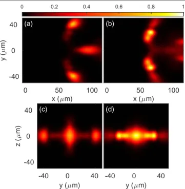
We are now in a position to follow the motion of the Rydberg atoms, which sets in as a consequence of the exciton forma-tion. Motion and exciton dynamics are modelled with a quantum–classical approach, described in appendixes Aand B. The four Rydberg atoms of the aggregate will move essentially unperturbed through the background gas[23]. This motion takes place in three-dimensional space and is governed by anisotropic resonant dipole–dipole interactions without any confinement. Initially atoms 1 and 2 repel each other as sketched infigure1. Eventually atom 2 comes closer to atoms 3 and 4 setting them into motion as well. The motion remains confined near the x−y-plane, facilitating observa-tions. The total atomic column densities(the total density in our case is just the sum over the spatial probability distribu-tions of each atom, see appendix D) after some time of free atomic motion have an interesting multi-lobed structure, shown in figure2, a central result of the present work. With the mechanical momentum transfer in mind, one would expect that atom 1 moves to the left infigure2(a) and atom 2 to the right. Both is indeed the case (at93 s atom 1 is nom longer within the range of thefigure). However, atom 2 has an elongated density profile along the x-axis at the final time. Moreover, one would expect the two atoms 3 and 4 to move outwards on the y-axis after the kick by atom 2. Although this is the case, the densities reveal two positions for each of them. The reason for this behaviour is that the electronic population gets distributed over two states(BO-surfaces) by traversing a CI at about 20μs. The CI occurs when atoms 2–4 nearly form an equilateral triangle. As a consequence, two BO-surfaces

Figure 2.Atomic densityn(r,t)(see appendixD) of the ﬁnal state

att=92.9 s, usingm q=ey. Shown are column densities,(a) in the

x–y plane, ¯ (n x y t, , ), and(b) in the y–z plane, ¯ (n y z t, , ), see appendixD. The white‘+’ mark the initial atomic positions. The maximal densities are set to 1.

4

The vectors qx, qy are chosen to complete a right-handed cartesian

coordinate system. They can be constructed by setting ≔

  ´ -á ñ qx a q a 2 a q, 2

andqy≔q´qx, in which a qcan be chosen arbitrarily, not changing the

(5)

are populated almost equally and exert different forces on the atoms. This explains the ‘double’—appearance of the final positions for atoms 3 and 4 and the blurredfinal position for atom 2. Figure 2(b) demonstrates that the entire dynamics indeed remains confined near the x–y-plane, which also facilitates the interpretation in terms of the BO-surfaces. Figure3 shows atomic densities segregated according to the two involved BO-surfaces and confirms the interpretation just given.

Note, that motion proceeds on the lower of the two surfaces when the CI was missed due to a conﬁguration asymmetric in y. This causes one of the y-dimer atoms to stay mostly at its initial position (maxima at x = 61 μm,

= 

y 18.5 μm), while the second receives a kick. In the density proﬁles this results in a total of four maxima for this surface, corresponding to kick and no-kick for both atoms 3 and 4. We discussed this phenomenology in more detail earlier[18,27].

The atomic motion in two orthogonal directions causes transfer of p-excitation from the initial m=0 orientation to the m= 1 orientations, as can be seen in ﬁgure 4. The ﬁgure shows the spatial distribution of the p-excitation seg-regated by magnetic quantum number, rexc,m(r,t), see appendixD. This is caused by the anisotropy of the dipole– dipole interactions, which is not present for one-dimensional geometries of the aggregate[17,19].

Optical conﬁnement of Rydberg atoms in one-dimen-sional traps along with a reduction of the electronic state space assumed in our related earlier work[20,27] constitute a signiﬁcant experimental challenge. The present results show that these restrictions are not required. It is simply the

symmetry of the initially prepared system which keeps the motion similarly planar and hence accessible. The successful splitting into different motional modes through the CI is a sensitive measure for the extent to which the atomic motion remains in a plane. Ourﬁndings suggest Rydberg aggregates as an experimental platform for the study of quantum chemical effects on much-inﬂated length and time scales with presently available technologies [15,34–36,49].

5. Considerations for an experiment

5.1. Experimental signatures

The total atomic density ofﬁgure2 is experimentally acces-sible if the focus positionsR( )₀n are sufﬁciently reproducible to allow averaging over many realisations. Additionally, one requires near single-atom sensitive position detection. A shot-to-shot position uncertaintys0in 3D within each laser focus is

already taken into account in our simulation. Recent advances in position sensitivefield ionisation enable ∼1 μm resolution, clearly sufficient for an image such as figure 2. The data for panel(b) could alternatively also be retrieved by waiting for atoms 3 and 4 to impact on a solid state detector. The background gas can also act as a probe for position and state of the embedded moving Rydberg atoms [15,30–33], offer-ing resolution sufficient for figure 2.

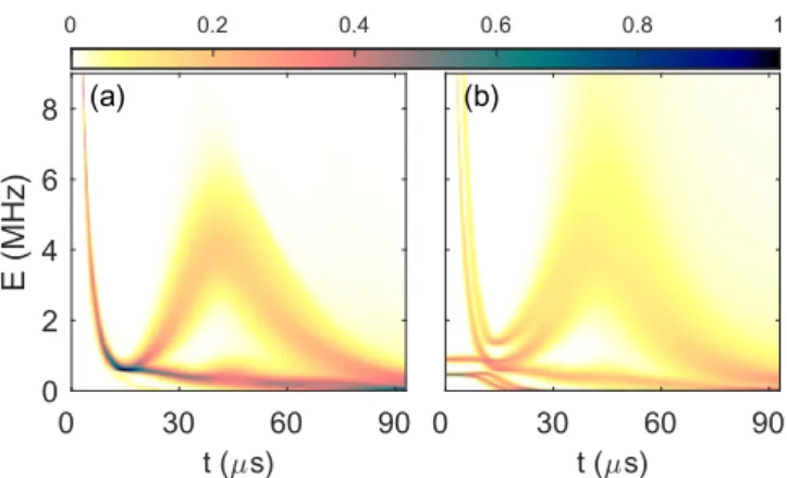
Non-adiabatic dynamics discussed here can not only be monitored in position space, but also in the excitation spec-trum of the system, similar to [34]. To obtain the time-resolved potential energy density (u E t, ), we bin the potential energy Us(t) of the currently propagated BO-surface s (see

appendixB) into a discretized energy grid E and average over all trajectories. Thereby, one can elegantly visualise electron dynamics on two BO-surfaces subsequent to CI crossing, as can be seen in ﬁgure5(a).

Observation ofu E t( , )could proceed by monitoring the time- and frequency-resolved outcome of driving the pd

transition. Similar techniques would allow an observation of the entire exciton spectrum of the system (with possibly unoccupied states), rather than only the currently populated state. The corresponding exciton density of states g E t( , ) analogous to u E t( , ), but now with all eigenenergies Uk Figure 3.As inﬁgure2, but with atomic density segregated according

to BOsurfaces: (a) and (c) second highest BOsurface, (b) and (d) fourth highest BOsurface. (a) and (b) column densities in the x–y-plane. (c) and (d) column densities in the y–z-plane. The global maximum for each column density is set to 1.

Figure 4.Spatial distribution of the(p, m)-excitation att=92.9 s.m Shown is the x–y column density, segregated by magnetic quantum numbers:(a)m= -1,rexc, 1_- (x y t, , ),(b) m=0,rexc,0(x y t, , )and

(c) m=1,r_exc,1(x y t, , ),see also appendixD. The global maximal density of excitation over all m-levels is set to 1.

4

(6)

binned instead of only the currently propagated surface Us,

is shown inﬁgure5(b).

5.2. Limits on laser waists and temperatures

Observable splitting of the dynamics onto different BO-sur-faces critically relies on guiding the atomic conﬁguration close to a CI location with the right spatial widths and velocities. The waist of the laser focus primarily determines the position uncertainty of the initial spatial conﬁguration of the aggregate, which impacts the population ratio of the relevant BOsurfaces. For larger waists, the distinct density features in the atomic density become blurred, such that it is no longer possible to clearly assign parts of the atomic density to dynamics along a particular BO surface. This is already the case for a waist size of σ0= 1 μm, as apparent from

ﬁgure6(b). An additional blurring is due to the temperature of the gas, through the velocity distribution.

However, the density profiles are more sensitive to changes in focus size than to temperature. This is verified in figure6: a doubling of the temperature fromT=1 Km (first row in figure 6) toT =2 Km (second row in figure6) still allows an identification of multi-BO features in the atomic densities for a laser waist size of s0= 0.5 mm , as apparent in

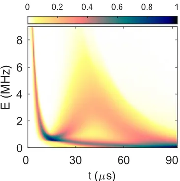
figure6(a). Only for temperatures aroundT =4 K can them multiple density features no longer be identified. Never-theless, even in this case, the CI still leaves its mark in the potential energy spectrum in the form of a distinct branching. This is even the case for a temperature ofT =4 K and am laser waist size of s0= 1 mm , as can be seen infigure7.

5.3. Perturbation by ground state atoms

We expect the dynamics of the embedded Rydberg aggregate discussed here not to be signiﬁcantly perturbed by its cold gas environment. Rydberg–Rydberg interactions substantially exceed elastic Rydberg ground-state atom interactions [50, 51] for separations d>200 nm, and dipole–dipole

excitation transport disregards ground state atoms[23]. Our

kinetic energies of (10 MHz), from dipole–dipole induced motion, are still low enough to render inelasticν or l changing collisions very unlikely [51], leaving molecular ion- or ion pair creation as main Rydberg excitation loss channel arising from collisions with ground state atoms [51, 52]. Thermal motion is even slower. When considering loss channels while assuming a background gas density of r =1 ´1012_cm−3_,

we can extrapolate experimental data from Rb[34] to infer a lifetime of about t= 530 s for the embedded Rydbergm aggregate (see appendix E). However, detrimentally large cross sections for the same processes were found in [51,52] for much larger densitiesρ. Further research on ionisation of fast Rydberg atoms within ultracold gases is thus of interest for the present proposal.

5.4. Alternative initialisation of the aggregate: trapping, cooling and excitation of atoms in optical tweezers

An alternative to initialise the Rydberg aggregate through direct excitation of atoms in the gas would be to individually trap four atoms in optical tweezers[53] at positionsR( )₀n, with trapping widths0, prior to Rydberg excitation, see e.g. [49].

Single atoms can be cooled to the vibrational ground state of optical tweezers [54], after which the atomic wave function approximately realises the ground state of a harmonic oscillator. The initial position uncertainty of the aggregate then is determined by the trapping frequenciesω of the optical tweezers. An uncertainty of s0= 0.5 mm for the location of

each atom, as used for the results in section 4, requires a trapping frequency, w p2 = (2p sM 02), of about 1 kHz, which is experimentally achievable[54]. A population of the vibrational ground state above 99% is reached for tempera-tures below 70 nK for this trapping frequency. This ground state yields a variance for the velocity,sv2=w 2M, of only

17% of the value corresponding to the ideal gas atT=1mK, as used in section4.

6. Switching of BO surfaces

The present system allows a simple handle deciding on which BO surface the system is initialised, and consequently to what extent the subsequent evolution involves CIs and non-adia-batic effects. This handle is the linear polarisation direction of the microwave for exciton creation, which selects the exciton state that is initially excited.

So far we have discussed the case q=ey. Choosing =

q ez instead allows the same sp excitation pulse to access a different initial BO-surface, with substantially less non-adiabaticity. This is shown in ﬁgure 8. The dramatic difference to the corresponding earlier results inﬁgures2and 5 can be viewed as a dependence on the magnetic quantum number of our initial state. With the microwave polarisation direction along ez, the third most energetic exciton is excited, which would contain m= 1 population using the previously chosen excitation direction.

Figure 5.Time-resolved spectra of(a) potential energy (u E t, )(as explained in the text) and (b) exciton density (g E t, )of all states. The maximum has been set to one for each density. To emphasise low density features, we plot u E t( , ) and g E t( , ), respectively. Such spectra are experimentally observable through time-resolved microwave spectroscopy[34].

(7)

7. Conclusions and outlook

In summary, controlled creation of a few Rydberg atoms in a cold gas of ground state atoms will allow to initiate coherent motion of the Rydberg atoms without external conﬁnement as

demonstrated here with the unconstrained motion of four Rydberg atoms, forming coupled excitonic BO surfaces. This enables non-adiabatic motional dynamics in assemblies of a few Rydberg excited atoms as an experimental platform for studies of quantum chemical processes inﬂated to con-venient time(microseconds) and spatial (micrometres) scales, with the perspective to shed new light on relevant processes such as ultra-fast vibrational relaxation [55] or reaction control schemes [56]. Experimental observables are atomic density distributions or exciton spectra.

The effects explored will be most prominent with light Alkali species, such as Li discussed here, but also the more common Rb can be used. Here, a slightly smaller setup would

Figure 6.Atomic density for increasing temperatures(top to bottom) and two different waist sizes of the excitation laser: (a) s0= 0.5 mm .

(b) s0= 1 mm . Shown are the x–y column density (left column) and y–z column density (right column) in (a) and (b), respectively.

Figure 7.Time-resolved spectrum of potential energy as inﬁgure5

but for temperatureT=4mK and laser waist size of s0= 1 mm .

Figure 8.Alternate dynamics for parameters as in section4but with microwave polarisation directionq=ez.(a) Column density in the

x–y plane att=92.9 s,m n x y t( , , ).(b) Potential energy density ( )

u E t, , plotted as inﬁgure5(a).

6

(8)

sufﬁciently accelerate the motion to ﬁt our scenario into the Rb system life-time. Rb would, however, pose a greater challenge for the theoretical modelling, making the inclusion of spin–orbit coupling necessary [44,45].

Since the CI in the arrangement discussed here is due to symmetry, it will occur regardless of the precise form of the dipole–dipole interactions. For instance, using a d-excitation (angular momentum l = 2) in a p-Rydberg aggregate should produce qualitatively similar results. For an s-excitation in a p-Rydberg aggregate, the results should even agree quanti-tatively, since a swap of p- and s-states leaves the dipole– dipole interaction unchanged. However, a symmetric splitting of population onto two surfaces always requiresﬁne-tuning of geometric parameters and would thus depend on details of interaction potentials.

Beyond the selective Rydberg atom activation discussed here, illuminating an entire 3D gas with a single Rydberg excitation laser, followed by microwave transitions to the p-state, should also quickly result in non-adiabatic effects. They would arise through the abundant number of CIs in random 3D Rydberg assemblies[20].

Acknowledgments

We acknowledge helpful discussions with Thomas Pohl.

Appendix A. Excitons and BO surfaces

The eigenstates of the electronic Hamiltonian equation(3) for aﬁxed arrangement R of atoms are termed Frenkel excitons [57]. We label them ∣j_k( )R ñand the corresponding eigen-energiesU Rk( ), deﬁned through

ˆ ( )∣j ( )ñ = ( )∣j ( )ñ ( )

Hel R k R Uk R k R . A.1 The Uk are also referred to as BO surfaces. Since our

electronic basis  has N3 elements for N atoms, the operator ˆ ( )

Hel R is represented by the3N´3N matrix

( ) ( ) ( ) ( ) ( ) ( )   = - - -⎛ ⎝ ⎜ ⎜ ⎞ ⎠ ⎟ ⎟ h h h h H R R R R R ... ... ... A.2 N N N N el 1, 1;1, 1 1, 1; ,1 ,1;1, 1 ,1; ,1

with ha, ; ,mbm¢( ) ≔R ápa,m H∣ ˆ ( )∣el R pb,m¢ ñ. The full elec-tronic wavefunction can be expanded in the eigenstates

∣y ñ =

å

˜ ∣j ( )ñ ( ) = c R , A.3 k N k k el 1 3

where the ˜cn are called the adiabatic expansion coefﬁcients. Since for each atom arrangement R the adiabatic eigenstates and the diabatic basis are linked via a unitary transformation, we can expand the electronic wavefunction also diabatically, i.e.

∣y ñ =

å å

∣p ñ ( ) a a a = =-c ,m , A.4 N m m el 1 1 1 ,

withca,m the diabatic coefﬁcients.

Appendix B. Propagation

The full dynamics is governed by the Hamiltonian

ˆ ( )= -

å

 + ˆ ( ) ( ) = H M H R R 2 . B.1 n N R 1 2 el n

For more than a couple of atoms, solving the time-dependent Schrödinger equation following fromequation (B.1) is not feasible in a reasonable time. However a quantum–classical propagation method, Tully’s fewest switching algorithm [58– 60], gives results in good agreement with the full propagation of the Schrödinger equation where possible [17,19,23,27]. In Tully’s fewest switching algorithm, the positions R of the atoms are treated classically according to Newton’s equation

( ) ( )

= -

MR¨ RUs R. B.2 Here, the atoms are subject to a mechanical potential that corresponds to a single eigenenergy Us of the electronic

Hamiltonian. The index s will undergo stochastic dynamics described below, for which one needs to calculate a large number of trajectories (solutions) of equation (B.2). The electronic state of the Rydberg aggregate is described quantum mechanically through the electronic Schrödinger equation

∣ ( ) ˆ ( ( ))∣ ( ) ( )

 ¶ y y

¶t t ñ =H R t t ñ

i el el el , B.3

whereR( )t , the solution of(B.2), enters as a parameter with Hel given in equation (A.2). We solve(B.3) by expanding

∣yel( )t ñin the diabatic basis , arriving at

˙ ( ) ( ( )) ( ) ( )

c t =H Rt c t

i el . B.4

To retain further quantum properties two features are added. Firstly, the atoms are randomly placed according to the Wigner distribution of the initial nuclear wavefunction and also receive a corresponding random initial velocity. In the end of the simulation, all observables have to be averaged over all realisations. Secondly, non-adiabatic processes are added as follows: The probability for a transition from surface l to surface k, is proportional to the non-adiabatic coupling vector

( )= áj ( ) ∣ ∣j( )ñ ( )

dkl R k R R l R . B.5

This coupling is realised in Tully’s algorithm by allowing for jumps of the index s, from an energy surface s=l to an energy surface s=k, during the propagation. The sequence of propagation is as follows:

(i) The initial positions of the atoms are randomly determined in accordance with the probability distribu-tionr(R,t=0 given in) (1). The initial velocities are also normally distributed R˙ ~(0,sv2), with the variance of velocity, s = k T Mv2 B , set in agreement

with an ideal, classical gas at temperature T.

(ii) The electronic Hamiltonian is diagonalized and we pick the electronic state with index k randomly according to the probability ∣áj_ini∣j_k(R0) ∣ñ2, where ∣ jiniñis the

(9)

(iii) The atomic positions are propagated one time step with equation (B.2), while states are propagated with equation(B.4).

(iv) We determine whether the surface index s undergoes a stochastic jump according to equation (B.5) (see [16] for the precise prescription).

(v) The new positions lead to new eigenstates and -energies, thus we repeat from(ii).

Appendix C. Microwave excitation to the initial electronic state

With a microwave  t0( ) that is linearly polarised in the q-direction, the aggregate can be excited from the state∣Sñto an exciton. The Hamiltonian of the microwave-atom coupling can approximately be written as

ˆ _{( )}₌_ _{( )}

_å

ˆ( ) ₍ ₎ a a = H t t d , C.1 N mw 0 1 0

where ˆd0( )a is the dipole operator of theαth atom projected

onto the polarisation direction of the microwave. The relative probability to excite from state ∣S ñwith all Rydberg elec-trons in(the same) s-state into a speciﬁc exciton state, ∣ j ñ_k ,

¹

k 0 with energy Uk, can be calculated via5

(∣ ∣ ) ∣ (∣ ∣ )∣ ( ) ∣ (∣ ∣ )∣ ( ) ( ) 

å

j j j ñ ñ = ñ ñ ñ ñ = S T S X U T S X U , , , , C.2 k k k l N l l 2 1 3 ₂

withT(∣Sñ,∣jñ) ≔ áS H∣ ˆmw( )∣t jñthe transition matrix

element from ∣S ñ ∣ jñdue to the microwave and X(E) the power spectral density of the microwave at energy E. Typi-cally we can assume X(E) to be a Gaussian, centred at the microwave frequency (energy)wmw. The transition matrix

element is given by (∣ ñ ∣jñ =)  ( )

å

( ) a a = T S , t c 3 , C.3 N 0 1 ,0 d

withca,0= ápa, 0∣jñthe diabatic expansion coefﬁcients of the exciton. The initial atomic conﬁguration is chosen, such that there are excitons localised on the x-dimer which provide repulsive interactions. According to(C.3), the microwave can only excite to excitons with excitation oriented along the microwave polarisation direction. Only forq Î{ey,ez}there is a single repulsive exciton, localised on the x-dimer, with even electronic symmetry

∣jñ »(∣p1, 0ñ +∣p2, 0ñ) 2 . (C.4) The latter is required for the transition according to(C.3) to be allowed such that we can initially excite to this state, ∣yel(t=0)ñ =∣jñ, by choosing a microwave frequency

ofwmw= 22.27 MHz.

Appendix D. Formulas for atomic density and spatial distribution of thep-excitation

In the following we specify several quantities used in the main text. The atomic density is deﬁned as

( ) ≔

å

ò

{ }r( )∣ ( ) = -= n t N t r, 1 d R R, , D.1 j N N j R r 1 1 j where ( ) ≔ ∣ ˆ ( )∣ ∣ ˆ ( )∣ ( )  

å

r p p á ñ = á ñ t t m t m R R R R R , ; , ; , D.2 k m k k nuc ,

is the probability distribution of the atomic positions R at time t. Note that we used the abbreviation ∣R;pk,mñ≔ ∣Rñ Ä∣ pk,mñ. The integration

ò

dN-1R{ }j is over all but the coordinates of the jth atom. The corresponding column den-sities are obtained by integrating out the direction which shall be removed. For instance, the atomic x–y column density is given by ¯ (n x y t, , )=

ò

dz n(r=(x y z, , ),t).

The m-level segregated spatial distributions of the p-excitation are deﬁned as

( ) ≔ ∣ ˆ ( )∣ ∣ ( ) { } 

ò

å

r p p ´ á ñ = -= t N m t m r R R R , 1 d ; , ; , D.3 m j N N j j j R r exc, 1 1 j

and the corresponding column densities are obtained in the same way as for the atomic density. In the context of Tully’s surface hopping, as described in appendixB, densities are calculated as follows: for each trajectory the relevant quantity is binned in a predeﬁned array and subsequently normalised by dividing through the number of trajectories. For the atomic density, the relevant quantity is the atomic conﬁguration of the aggregate, whereas for the spatial excitation density, before binning, the position of each atom is weighted with the probability that the respective atom carries excitation. For more details of the pro-cedure, see the supplemental information of[27].

Appendix E. Inelastic interactions with the background gas

For the scenario proposed here, Rydberg excited atoms with

n = 80 in l=0, 1 states move through a background gas of ground state atoms with density r = 1´1012_cm−3_{at a}

max-imal velocity of about vini~ Uini(R0) 2 »0.85 m s–1. We can deduce a maximal cross-section for ionising collisions between Rydberg atoms and ground state atoms of

( )

s n = 610 nm2

at n = 60 from experiment [34]. Assuming scaling with the size of the Rydberg orbit[52], we extrapolate this value to our n = 80, thuss(80)=s(60 80 60 10)( )2 3_{; nm}2_.

The total decay rate of our four atom system is then G = Gtot 2 coll+ G4 0, with spontaneous decay rate G0 and

collisional decay rate Gcollfor single atoms. We have assumed

that only two atoms ever move with the fastest velocity. UsingGcoll= vr inis(80), weﬁnally arrive at a total life-time

t=1 G =tot 530 sm as quoted in the main text.

5

We useUkwmw.

8

(10)

References

[1] Gallagher T F 1994 Rydberg Atoms (Cambridge: Cambridge University Press)

[2] Browaeys A, Barredo D and Lahaye T 2016 J. Phys. B: Atom. Mol. Opt. Phys.49 152001

[3] Jaksch D et al 2000 Phys. Rev. Lett.85 2208

[4] Lukin M D et al 2001 Phys. Rev. Lett.87 037901

[5] Urban E et al 2009 Nat. Phys.5 110

[6] Gaëtan A et al 2009 Nat. Phys.5 115

[7] Lesanovsky I and Garrahan J P 2013 Phys. Rev. Lett.111 215305

[8] van Bijnen R M W and Pohl T 2015 Phys. Rev. Lett.114 243002

[9] Glaetzle A W et al 2015 Phys. Rev. Lett.114 173002

[10] Wilk T et al 2010 Phys. Rev. Lett.104 010502

[11] Müller M M et al 2014 Phys. Rev. A89 032334

[12] Mülken O et al 2007 Phys. Rev. Lett.99 090601

[13] Barredo D et al 2015 Phys. Rev. Lett.114 113002

[14] Bettelli S et al 2013 Phys. Rev. A88 043436

[15] Günter G et al 2013 Science342 954

[16] Ates C, Eisfeld A and Rost J M 2008 New J. Phys.10 045030

[17] Wüster S, Ates C, Eisfeld A and Rost J M 2010 Phys. Rev. Lett.105 053004

[18] Leonhardt K, Wüster S and Rost J M 2016 Phys. Rev. A93 022708

[19] Möbius S et al 2011 J. Phys. B: At. Mol. Opt. Phys.44 184011

[20] Wüster S, Eisfeld A and Rost J M 2011 Phys. Rev. Lett.106 153002

[21] Wüster S, Ates C, Eisfeld A and Rost J M 2011 New J. Phys.

13 073044

[22] Zoubi H, Eisfeld A and Wüster S 2014 Phys. Rev. A89 053426

[23] Möbius S et al 2013 Phys. Rev. A88 012716

[24] Wüster S et al 2013 Phys. Rev. A88 063644

[25] Genkin M et al 2014 J. Phys. B: At. Mol. Opt. Phys.47 095003

[26] Möbius S et al 2013 Phys. Rev. A87 051602

[27] Leonhardt K, Wüster S and Rost J M 2014 Phys. Rev. Lett.113 223001

[28] Domcke W, Yarkony D R and Köppel H 2004 Conical Intersections(Singapore: World Scientiﬁc)

[29] White A J, Peskin U and Galperin M 2013 Phys. Rev. B88 205424

[30] Olmos B, Li W, Hofferberth S and Lesanovsky I 2011 Phys. Rev. A84 041607(R)

[31] Günter G et al 2012 Phys. Rev. Lett.108 013002

[32] Schönleber D W et al 2015 Phys. Rev. Lett.114 123005

[33] Schempp H et al 2015 Phys. Rev. Lett.115 093002

[34] Celistrino Teixeira R et al 2015 Phys. Rev. Lett.115 013001

[35] Thaicharoen N, Schwarzkopf A and Raithel G 2015 Phys. Rev. A92 040701(R)

[36] Thaicharoen N, Gonçalves L F and Raithel G 2016 Phys. Rev. Lett. 116 213002

[37] Fioretti A et al 1999 Phys. Rev. Lett.82 1839

[38] Li W, Tanner P J and Gallagher T F 2005 Phys. Rev. Lett.94 173001

[39] Mudrich M et al 2005 Phys. Rev. Lett.95 233002

[40] Marcassa L G, de Oliveira A L, Weidemüller M and Bagnato V S 2005 Phys. Rev. A71 054701 [41] Nascimento V A et al 2006 Phys. Rev. A73 034703

[42] Amthor T et al 2007 Phys. Rev. Lett.98 023004

[43] Amthor T, Reetz-Lamour M, Giese C and Weidemüller M 2007 Phys. Rev. A76 054702

[44] Park H et al 2011 Phys. Rev. A84 022704

[45] Park H, Shuman E S and Gallagher T F 2011 Phys. Rev. A84 052708

[46] Lühmann D-S, Weitenberg C and Sengstock K 2015 Phys. Rev. X,5 031016

[47] Goy P, Liang J and Haroche S 1986 Phys. Rev. A34 2889

[48] Robicheaux F, Hernandez J V, Topcu T and Noordam L D 2004 Phys. Rev. A70 042703

[49] Nogrette F et al 2014 Phys. Rev. X,4 021034

[50] Greene C H, Dickinson A S and Sadeghpour H R 2000 Phys. Rev. Lett.85 2458

[51] Balewski J B et al 2013 Nature502 664

[52] Niederprüm T et al 2015 Phys. Rev. Lett.115 013003

[53] Grünzweig T, Hilliard A, McGovern M and Andersen M F 2010 Nat. Phys.6 951

[54] Kaufman A M, Lester B J and Regal C A 2012 Phys. Rev. X2 041014

[55] Perun S, Sobolewski A L and Domcke W 2005 Chem. Phys.

313 107

[56] Epshtein M, Yifrach Y, Portnov A and Bar I 2016 J. Phys. Chem. Lett.7 1717

[57] Frenkel J 1931 Phys. Rev.37 17

[58] Tully J C and Preston R K 1971 J. Chem. Phys.55 562

[59] Hammes-Schiffer S and Tully J C 1994 J. Chem. Phys.101 4657

[60] Barbatti M 2011 Wiley Interdiscipl. Rev. Comput. Mol. Sci.