ENVIRONMENT
a thesis
submitted to the department of industrial engineering
and the institute of engineering and science
of bilkent university
in partial fulfillment of the requirements
for the degree of
master of science
By
Taylan ˙Ilhan
September, 2002
I certify that I have read this thesis and that in my opinion it is fully adequate, in scope and in quality, as a thesis for the degree of Master of Science.
Assoc. Prof. M. Selim Akt¨urk(Advisor)
I certify that I have read this thesis and that in my opinion it is fully adequate, in scope and in quality, as a thesis for the degree of Master of Science.
Assist. Prof. Oya Ekin Kara¸san
I certify that I have read this thesis and that in my opinion it is fully adequate, in scope and in quality, as a thesis for the degree of Master of Science.
Assoc. Prof. M. C¸ elebi Pınar
Approved for the Institute of Engineering and Science:
Prof. Dr. Mehmet B. Baray Director of the Institute
TIMES IN A CNC ENVIRONMENT
Taylan ˙Ilhan
M.S. in Industrial Engineering Supervisor: Assoc. Prof. M. Selim Akt¨urk
September, 2002
Flexible manufacturing systems give a manufacturer some capabilities to con-sider and solve different manufacturing problems simultaneously instead of one by one in a sequential manner. Using those makes her more competitive in the market. One of those capabilities is controllable processing times. By using this capability, the due date requirements of customers can be satisfied much more ef-fectively. Processing times of the jobs in a CNC machine can be easily controlled via machining conditions such that they can be increased or decreased at the ex-pense of tooling cost. In this study, we consider the problem of scheduling a set of jobs by minimizing the sum of total weighted tardiness, tooling and machining costs on a single CNC machine. This problem is NP-hard since the total weighted tardiness problem is NP-hard alone. Moreover, the problem is non-linear because of the nature of the tooling cost. We proposed a DP-based heuristic to solve the problem for a given sequence and designed a local search algorithm that uses it as a base heuristic.
Keywords: Scheduling, Single Machine, Total Weighted Tardiness, Machining
Conditions, Controllable Processing Times, Heuristics. iii
¨
OZET
CNC ORTAMINDA KONTROL ED˙ILEB˙IL˙IR ¨
URET˙IM
ZAMANLARIYLA C
¸ ˙IZELGELEME
Taylan ˙Ilhan
End¨ustri M¨uhendisli˘gi, Y¨uksek Lisans Tez Y¨oneticisi: Assoc. Prof. M. Selim Akt¨urk
Eyl¨ul, 2002
Esnek ¨uretim sistemleri bir ¨ureticiye farklı ¨uretim problemlerini tek tek sırayla de˘gil aynı anda ¸c¨ozebilmesini sa˘glayan kabiliyetler verir. Bu kabiliyetleri kullan-mak onu pazarda ¸cok daha rekabet¸ci bir hale getirir. Bu kabiliyetlerden birisi de bilgisayar sistemleri ¨uzerinden kontrol edilebilir ¨uretim zamanlarıdır. Bu kabiliyeti kullanarak m¨u¸sterilerin teslim zamanı gereksinimleri daha efektif bir ¸sekilde kar¸sılanabilir. Bir CNC makinasında i¸slenecek olan i¸slerin ¨uretim zaman-ları i¸sleme ko¸sulzaman-ları ¨uzerinden kontrol edilebilir, yani kesici u¸c maliyeti kar¸sılı˘gında arttırılabilir ya da azaltılabilir. Bu ¸calı¸smada, toplam a˘gırlıklı gecikme, kesici u¸c ve i¸sleme maliyetlerini enazlayarak bir grup i¸sin ¸cizelgelenmesini g¨oz¨on¨une aldık. Tek ba¸sına toplam a˘gırlıklı gecikme problemi NP-zor olmasından dolayı, bizim inceledi˘gimiz problem de NP-zor’dur. Ayrıca, kesici u¸c maliyetinin do˘gasından dolayı da problem do˘grusal de˘gildir. Bu ¸calı¸smamızda sırası verilmi¸s i¸slerin ¸cizelgelenmesi i¸cin DP temelli bir y¨ontem ve bu y¨ontemi temel algoritma olarak kullanan bir genetik problem uzayı algoritması tasarladık.
Anahtar s¨ozc¨ukler : C¸ izelgeleme, Toplam A˘gırlıklı Gecikme, ˙I¸sleme Ko¸sulları,
Kontrol Edilebilir ¨Uretim Zamanları, Yordamlama.
I would like to express my deepest gratitude to Assoc. Prof. Selim Akt¨urk for his invaluable guidance, encouragement and enthusiasm which he inspired on me during my study.
I am grateful to Assist. Prof. Oya Ekin Kara¸san for accepting to read and review this thesis and her valuable comments and suggestions.
I am also indebted to Assoc. Prof. M. C¸ elebi Pınar for the valuable remarks and guidance in his review.
I am indebted to Ayten T¨urkcan for sharing her creative ideas and comments with me.
I also would like to thank to my dear Filiz G¨urtuna for her invaluable com-ments, suggestions and support during my study.
I would like to thank to Burkay Gen¸c for his valuable friendship.
Finally, I would like to thank to my family for their support to bring this thesis to an end.
Contents
1 Introduction 1
2 Literature Review 4
2.1 Tool Management and Machining Conditions . . . 4
2.2 Scheduling . . . 10
2.2.1 Controllable Processing Times . . . 10
2.2.2 The Total Weighted Tardiness . . . 13
2.3 Summary . . . 15
3 Problem Statement and Modeling 17 3.1 Problem Definition . . . 17
3.1.1 Assumptions and Notations . . . 18
3.2 Mathematical Modeling . . . 19
3.2.1 SMOP and Lower & Upper Bounds for Processing Times . 20 3.2.2 Cost Items of the Problem . . . 22
3.2.3 Mathematical Formulation . . . 23 vi
3.3 Summary . . . 25
4 Proposed Heuristic Algorithms 26 4.1 The Sequential Algorithm . . . 27
4.2 The Proposed Simultaneous Algorithm . . . 27
4.3 The Proposed DP-based Heuristic . . . 32
4.3.1 Explanation of Graph Generation . . . 34
4.3.2 Explanation of State Generation . . . 38
4.4 Complexity Analysis . . . 47
4.5 Summary . . . 48
5 An Illustrative Example 49 6 Experimental Design 57 6.1 Experimental Settings . . . 57
6.2 Results for the Problem for a Given Sequence . . . 59
6.3 Local Search Parameters and Results . . . 62
6.4 Summary . . . 66
7 Conclusion 67 7.1 Contributions . . . 67
CONTENTS viii
A Construction of Ri(∆i) 76
A.1 State (A,1) . . . 77
A.2 State (A,2) . . . 78
A.3 State (B,2) . . . 79
A.4 States (A,3), (C,1), (C,3) . . . 80
A.5 States (B,1), (C,2), (B,3) . . . 81
B Results for The Problem with a Given Sequence 83 C Results for The Original Problem 93 C.1 Cost Values . . . 94
C.2 CPU Time Values . . . 96
D Statistical Analysis of Results 98 D.1 Analysis of The Problem with a Given Sequence . . . 98
D.2 Analysis of The Original Problem . . . 103
4.1 The cost items for each job . . . 39 4.2 0 ≤ ∆i < r[k]− mink . . . 42 4.3 r[k+1]− mink≤ ∆ i < r[k+1]− mink+1 . . . 42 4.4 r[k]− mink ≤ ∆ i < r[k+1]− mink . . . 43
4.5 Two lines that form concave shape . . . 44
4.6 The illustration of possible total costs for two tardiness lines . . . 46 4.7 Possible combinations of locations of ranges for two tardiness lines
and information about cost items corresponding to each line . . . 47
A.1 The illustration of combination (A, 1) . . . 78
List of Tables
5.1 Problem data . . . 49
6.1 Experimental design factors . . . 58
6.2 Technical coefficients and parameters . . . 59
6.3 Summary results for the problem with given sequence . . . 60
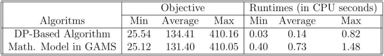
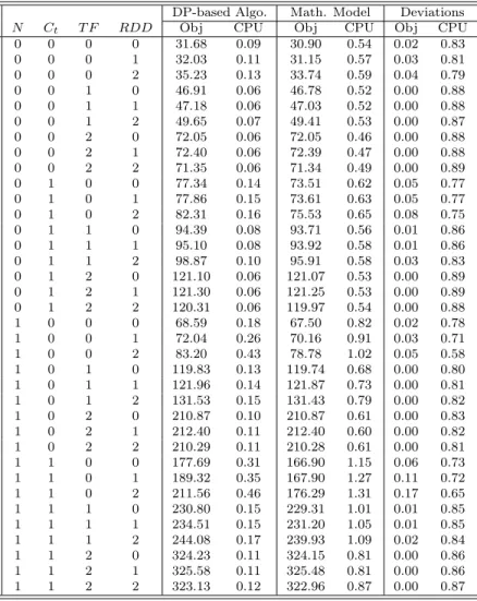
6.4 Comparison of DP-based heuristic with Math model in GAMS . . 61
6.5 Definitions and levels of PSGA parameters for the sequential and the proposed simultaneous algorithms . . . 63
6.6 Summary results of PSGA’s for the problem . . . 63
6.7 Deviations of Algorithms for the original problem with respect to each other . . . 64
6.8 Comparison of the sequential and the proposed simultaneous algo-rithms . . . 65
D.1 Paired samples statistics for DP-based algorithm and Math Model solved in GAMS . . . 98
D.2 Paired samples correlations for DP-based algorithm and Math Model solved in GAMS . . . 98
D.3 Paired samples test results for DP-based algorithm and Math Model solved in GAMS . . . 98 D.4 Test of Between-Subjects Effects for the cost values of DP-based
algorithm and Math Model solved in GAMS . . . 99
D.5 Estimated Marginal Grand Mean for the cost values of two stage
algorithm and proposed PSGAs . . . 99
D.6 Estimated Marginal Mean by the factor N for the cost values of
DP-based algorithm and Math Model solved in GAMS . . . 99
D.7 Estimated Marginal Mean by the factor Ctfor DP-based algorithm
and Math Model solved in GAMS . . . 99
D.8 Estimated Marginal Mean by the factor T F for DP-based algo-rithm and Math Model solved in GAMS . . . 100 D.9 Estimated Marginal Mean by the factor RDD for DP-based
algo-rithm and Math Model solved in GAMS . . . 100 D.10 Paired samples statistics for CPU times of DP-based algorithm
and Math Model solved in GAMS . . . 100 D.11 Paired samples correlations for CPU times of DP-based algorithm
and Math Model solved in GAMS . . . 100 D.12 Paired samples test results for CPU times of DP-based algorithm
and Math Model solved in GAMS . . . 100 D.13 Test of Between-Subjects Effects for the cost values of DP-based
algorithm and Math Model solved in GAMS . . . 101 D.14 Estimated Marginal Grand Mean for the CPU times of two stage
LIST OF TABLES xii
D.15 Estimated Marginal Mean by the factor N for the CPU times of DP-based algorithm and Math Model solved in GAMS . . . 101
D.16 Estimated Marginal Mean by the factor Ct for the CPU times of
DP-based algorithm and Math Model solved in GAMS . . . 101 D.17 Estimated Marginal Mean by the factor T F for the CPU times of
DP-based algorithm and Math Model solved in GAMS . . . 102 D.18 Estimated Marginal Mean by the factor RDD for the CPU times
of DP-based algorithm and Math Model solved in GAMS . . . 102 D.19 Paired samples statistics for the sequential algorithm and proposed
PSGAs . . . 103 D.20 Paired samples correlations for the sequential algorithm and
pro-posed PSGAs . . . 103 D.21 Paired samples test results for PSGA parameter sets . . . 103 D.22 Test of Between-Subjects Effects for the cost values of sequential
algorithm and proposed PSGAs . . . 104 D.23 Estimated Marginal Grand Mean for the cost values of the
sequen-tial algorithm and proposed PSGAs . . . 104 D.24 Estimated Marginal Mean by the factor N for the cost values of
the sequential algorithm and proposed PSGAs . . . 104
D.25 Estimated Marginal Mean by the factor Ct for the cost values of
the sequential algorithm and proposed PSGAs . . . 104 D.26 Estimated Marginal Mean by the factor T F for the cost values of
the sequential algorithm and proposed PSGAs . . . 105 D.27 Estimated Marginal Mean by the factor RDD for the cost values
D.28 Paired samples statistics for CPU times of the sequential algorithm and proposed PSGAs . . . 105 D.29 Paired samples correlations for the CPU times of the sequential
algorithm and proposed PSGAs . . . 105 D.30 Paired samples test results for the CPU times of the sequential
algorithm and proposed PSGAs . . . 106 D.31 Test of Between-Subjects Effects for the CPU times of the
sequen-tial algorithm and proposed PSGAs . . . 106 D.32 Estimated Marginal Grand Mean for the CPU times of the
sequen-tial algorithm and proposed PSGAs . . . 106 D.33 Estimated Marginal Mean by the factor N for CPU times of the
sequential algorithm and proposed PSGAs . . . 106
D.34 Estimated Marginal Mean by the factor Ct for the CPU times of
the sequential algorithm and proposed PSGAs . . . 107 D.35 Estimated Marginal Mean by the factor T F for the CPU times of
the sequential algorithm and proposed PSGAs . . . 107 D.36 Estimated Marginal Mean by the factor RDD for the CPU times
Chapter 1
Introduction
Buyer-vendor relationship plays an important role in business. Usually, buyers desire reliable time delivery for meeting their schedules. From the perspective of the vendors, each buyer has a different priority. All of these require vendors to consider weighted tardiness problem in their scheduling decisions. If a manu-facturer has a flexible manufacturing system, in addition to its other capabilities she also gains a capability to be more competitive in meeting customer due date requirements. This capability is to be able to control processing times, which is a readily available feature on modern CNC machines.
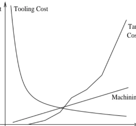
Processing times in a CNC machine are controlled by machining conditions, for example feed rate and cutting speed in a turning machine. We can increase or decrease the processing time of a job by changing the machining conditions. However, there is a cost which is incurred when we increase the processing speed. It is the tooling cost, to which a manufacturer should always pay attention to use CNC machines effectively. Gray et al. [22] and Veeramani et al. [53] give extensive surveys on the tool management issues of FMS, and emphasize that the lack of tooling considerations has resulted in the poor performance of these systems.
In the literature, the interaction between determining machining conditions and solving single machine weighted tardiness problem is never analyzed up to
now. Moreover, in the industry, they are considered as decisions at two different levels of FMS hierarchy. Machining conditions are determined in the design level and scheduling problems are solved in the operational level. To convert the capability of controlling processing times to an advantage for a manufacturer, instead of solving these problems one by one in a sequential manner we propose a solution methodology for solving them together by considering the relations between them.
In this study, we consider the problem of scheduling a set of jobs by minimizing the sum of total weighted tardiness, tooling and machining costs on a single CNC machine. This problem is NP-hard since the total weighted tardiness problem is NP-hard alone. Moreover, the problem is non-linear because of the nature of the tooling cost. Processing times of the jobs are controllable because they depend on the machining conditions. Thus, finding an efficient algorithm that solves the problem exactly is almost impossible.
In our study, we first develop an efficient Dynamic Programming(DP) based heuristic algorithm that considers interactions among the jobs using a con-tributed cost function. The proposed algorithm minimizes the summation of total weighted tardiness, tooling and machining costs over a given sequence. We then employ a problem space heuristic based on a local search algorithm that uses the proposed algorithm as a base heuristic to determine the processing time of each job and the schedule of all jobs simultaneously to minimize the stated objective function. At each stage of the base algorithm, we generate a set of pro-cessing time alternatives for each job in a recursive equation (that corresponds to states in a DP format) in a backward DP algorithm. After finding the optimal processing time for the first job in the sequence, it generates the optimal process-ing times for the rest of the jobs by usprocess-ing the recursive equations and alternative states of each job in a forward DP algorithm.
CHAPTER 1. INTRODUCTION 3
We compared computationally our DP-based heuristic with mathematical for-mulation of the problem for a given sequence, and found that our heuristic de-creases CPU times dramatically at the expense of losing little from solution qual-ity. Also the computational results over the original problem show that our pro-posed local search algorithm produces solutions with much higher quality when compared to the sequential algorithm that determines machining conditions first and then solves the scheduling problem for the total weighted tardiness criterion. Although, CPU times of our algorithm are higher than the ones of the sequen-tial algorithm, they are in acceptable ranges considering the improvement in the solution quality.
In the next chapter, we present a literature review on machining conditions optimization in tool management, controllable processing times and weighted tardiness concerns in scheduling literature. In Chapter 3, we define the scope of this study and give the mathematical formulations of the problem. In Chapter 4, we introduce our proposed heuristic approaches and in Chapter 5 we present an illustrative example for our proposed DP-based heuristic. Experimental design and computational results are given in Chapter 6. Finally, we conclude in Chapter 7 giving final remarks and future research directions.
Literature Review
In literature, both tool management issues and scheduling problems have been extensively researched. However, they are considered separately. The interaction between them is ignored. In this section, we give a short literature review related to tool management, and scheduling with controllable processing times and with total weighted tardiness criterion, 1||PwiTi.
In order to give the related literature in an organized manner, we will start with the tool management and machining condition issues in the following section. Then, we will give the literature on scheduling with controllable processing times and with weighted tardiness criterion. Finally, we will conclude by mentioning the drawbacks of the current literature that motivate us for this study.
2.1
Tool Management and Machining
Condi-tions
Flexibility is a key requirement in manufacturing systems to cope with modern market environment which is characterized by diverse products, high quality and short lead time. Crama and Klundert [12] define the most vital component of flexibility as “the ability of machines to perform various operations on various
CHAPTER 2. LITERATURE REVIEW 5
products or parts”. The term “flexible” is generally used to describe two aspects of the system [44]: (1) the ability to use alternative routings through the machines to perform a given set of operations, and (2) the ability to simultaneously machine different part types. This flexibility is achieved by the use of CNC machines which are capable of carrying multiple tools. Also, the versatility of an FMS is achieved by equipping each machine with a tool magazine. This magazine can hold a set of tools which the machine can use to perform a succession of operations while incurring low setup costs when switching from one tool to another. In reality, FMSs are only capable of processing a finite family of parts at any given time. The flexibility or randomness is limited by the allocation of supporting resources such as pallets, fixture, and tools. As FMSs expand into the low volume, high variety production environment, the number of pallets, fixture, and tools and the amount of handling of these resources are increased. The management of these resources, especially the tooling which accounts for a high percentage of the operating costs of an automated manufacturing environment, is an absolute must. Therefore the models including tool management improves the productivity for an FMS.
Due to its direct impact on system performance, its dynamic nature and the large amount of information involved, the tooling problem has been considered as one of the most important and complicated issues in automated manufactur-ing. Proper tool management ensures that the correct tools are on the appro-priate machines at the right time so that the desired quantities of workpieces are manufactured and the machine utilizations are maintained. Tool inventory, maintenance and distribution issues determine the quantity of work produced and system utilizations.
Tool management is an important area of research which has been extensively studied for nearly a hundred years, since Taylor [50] first recognized in 1907 that the machining conditions should be optimized to minimize the machining cost. Malakooti and Deviprasas [35] list vital contributions on parameter selection in metal cutting from 1907 up to 1985 in their paper.
It is stated by Stecke [46] and Gray et al. [22] that approximately 50 percent of U.S. annual expenditures on manufacturing is in the metal working industry,
and two thirds of metal working is metal cutting. Besides being a critical issue in factory integration, tool management has direct cost implications. Kouvelis [30] reports in his study that tooling accounts for 25 percent to 30 percent of both fixed costs and variable costs of production in an automated machining environment. The reason for such a high contribution of the tooling to the total manufacturing cost is related to the high material removal rate in metal cutting processes, and the consequent increased tool consumption rates and tool replacement frequencies.
Kaighobadi and Venkatesh [27] state that the lack of attention to cutting tool related issues is a main reason for making an FMS inflexible in practice. Gray et al. [22] and Veeramani et al. [53] give extensive surveys on the tool management issues in automated manufacturing systems, and emphasize that the lack of tool management considerations has resulted in the poor performance of these systems.
The optimization of the machining conditions for a single operation is a well known problem, where the decision variables are usually the cutting speed and the feed rate. These conditions are the key to economical machining operations. Knowledge of optimal cutting parameters for machining operations is required for process planning of metal cutting operations. Numerous models have been developed with the objective of determining optimal machining conditions.
Malakooti and Deviprasas [35] formulate a metal cutting operation, specif-ically for a turning operation, as a discrete multiple objective problem. The objectives are to minimize cost per part, production time per part, and rough-ness of the work surface, simultaneously. They discuss a heuristic gradient-based multiple criteria decision making approach which they apply to parameter se-lection in metal cutting. For the metal cutting problem, they show how effi-cient alternatives can be generated by a discrete variable approach and how the gradient-based multiple objective approach can be implemented to obtain the most preferred alternative. They also discuss their software package for micro-computers as a decision support system for parameter selection. They compare their computer aided machine parameter selection (CAMPS) package to some of the computer packages (used in 1987) in the market.
CHAPTER 2. LITERATURE REVIEW 7
Duffuaa et al. [15] compare the results of a number of gradient based opti-mization algorithms with different machining models. Their approach is limited because of the use of gradient based methods which are not ideal for non-convex problems. They conclude that the generalized reduced gradient method is the most suitable for solving machining optimization models.
Petropoulos [39] has used geometric programming for optimization of machin-ing parameters. Multi-pass turnmachin-ing optimization has been addressed by Ermer and Kromodihardjo [19]. They use a combination of linear and geometric pro-gramming.
Iwata et al. [26] use a stochastic approach to solve for optimal machining parameters. Eskicioglu and Eskicioglu [20] demonstrate the use of non-linear programming for machining parameter optimization. Hati and Rao [23] use se-quential unconstrained minimization technique (SUMT) to solve a multi-pass turning operation.
Khan et al. [29] study machining condition optimization by genetic algorithms and simulated annealing. Although nonlinear and non-convex machining models developed with the objective of determining optimal cutting conditions are tra-ditionally solved using gradient based algorithms, they study three non gradient based stochastic optimization algorithms and test their efficiency in solving sev-eral benchmark machining models which are complex because of non-linearities and non-convexity.
Stori et al. [47] integrate process simulation in machining parameter opti-mization and propose a methodology for incorporating simulation feedback to fine-tune analytic models during optimization process. They present a non-linear programming (NLP) optimization technique used to select process parameters based on closed-form analytical constraint equations relating to critical design requirements and execute simulation using these process parameters, providing predictions of the critical state variables. Then, they dynamically adapt con-straint equation parameters using the feedback provided by the simulation pre-dictions. They repeat this sequence until local convergence between simulation and constraint equation predictions has been achieved.
Thomas et al. [51] emphasize the importance of choice of optimized cutting tool parameters to control the required surface quality. Surface finish is an im-portant requirement for many turned work pieces in machining operation. The authors dealt with the interactions between the cutting parameters and surface roughness. They investigated the effects of tool vibration on the resulting surface roughness in the dry turning operation of carbon steel. They chose a full factorial design that allowed to consider the three-level interactions between the cutting parameters (cutting speed, feed rate, tool nose radius, depth of cut, tool length, and workpiece length) on the two measured dependent variables (surface rough-ness and tool vibration). Their results show that the factors having the greatest influence on surface roughness are the second order interactions between cutting speed and tool nose radius, along with third-order interaction between feed rate, cutting speed and depth of cut. They had the best surface finish at a low feed rate, a large tool nose radius and a high cutting speed. They concluded that feed rate and tool nose radius produced the most important effects on surface roughness, followed by cutting speed.
Kyoung et al. [32] emphasized the importance of selecting tool size, tool path, cutting width at each tool path properly and calculating the machining time for optimal process planning. Since other factors depend on the tool size, it is the most important factor in their problem. They presented a method for selecting optimal tools for pocket machining for the components of injection mold. They applied the branch and bound method to select the optimal tools which minimize the machining time by using the range of feasible tools and the breadth-first search.
These models consider only the contribution of machining time and tooling cost to the total cost of operation, and they usually ignore the contribution of the non-machining time components to the operating cost, which could be significant for the multiple operation case. All of the time consuming events except the actual cutting operation are denoted as non-machining time components. Ba-sic setup, tool interchanging, tool replacing, workpiece loading-unloading, tool
CHAPTER 2. LITERATURE REVIEW 9
tuning, tool approach and stabilization etc., are the typical examples of machining events. Machining conditions are the main determinants of these non-machining time components. These studies also exclude the tooling issues such as the tool availability and the tool life capacity limitations. Therefore, their results might lead to infeasibilities due to tool contention among operations for a limited number of tool types [37].
Akt¨urk and Avcı [4] proposed a solution procedure to make tool allocation and machining conditions selection decisions simultaneously. They also take into account the related tooling considerations of tool wear, tool availability, and tool replacing and loading times, since they affect both the machining and non-machining time components, hence the total cost of manufacturing. In their study, they extend single machining operation problem (SMOP) formulation by adding a new tool life constraint which enables them to include tooling issues like tool wear and tool availability. Furthermore, they propose a new cost measure to exploit the interaction between the number of tools required with the machining, tool replacing and loading times, and tool waste cost in conjunction with the optimum machining conditions for alternative operation-tool pairs. Consequently, they prevent any infeasibility that might occur for the tool allocation problem at the system level due to tool contention among tool life restrictions through a feedback mechanism.
Akt¨urk and ¨Onen [6] proposed a new algorithm to solve lot sizing, tool alloca-tion and machining condialloca-tions optimizaalloca-tion problems simultaneously to minimize the total production cost in a CNC environment. They integrated the system, machine and tool level decisions for production of multiple parts consisting of multiple operations. This way, they avoid any infeasibility that may occur due to tool and machine hour availability limitations.
In a recent study, Akt¨urk [3] developed an exact approach to determine the optimum machining conditions and tool allocation decisions simultaneously to minimize the total production cost on a CNC turning machine where alternative tools can be used for each operation. He emphasized the tool management issues
at the tool level such as the optimum machining conditions and tool selection-allocation decisions considering the tool life, machining operations and tool avail-ability constraints. He presented a new mathematical model and proposed an efficient solution procedure to determine concurrently the optimal machining con-ditions of cutting speed and feed rate, the optimal operation-tool assignment and optimal allocation of tools.
2.2
Scheduling
Scheduling is concerned with determining the sequence in which available work should be processed to optimize system performance.
Standard formulations of the scheduling problem assume that job processing times are fixed and known in advance of scheduling. In practice, processing times are often a function of the amount and mix of resource inputs allocated to a job. These resources can vary depending on the system. For instance, in a production facility composed of CNC machines, machine cutting speed and feed rate are effective parameters changing the processing times and tool usage rates. In a relatively labor-intensive systems, processing time typically depend on the number and type of the workers allocated to the system (Daniels et al. [13]).
2.2.1
Controllable Processing Times
Processing time control and its impact on sequencing decisions and operational performance have received limited attention in the scheduling literature. Some models for single-processor systems have been developed and studied concerning controllable processing times. Extensions to parallel-machine environments are also addressed by researchers. A survey of the literature up to 1990 can be found in Nowicki and Zdrzalka [36].
Daniels and Sarin [14] consider the problem of joint sequencing and resource allocation when the scheduling criterion of interest is the number of tardy jobs
CHAPTER 2. LITERATURE REVIEW 11
and derive theoretical results that aid in developing the trade-off curve between the number of tardy jobs and the total amount of allocated resource.
Panwalker and Rajagopalan [38] consider the static single machine sequencing problem with a common due date for all jobs in which job processing times are controllable with linear costs. They develop a method to find optimal processing times and an optimal sequence to minimize a cost function containing earliness cost, tardiness cost and total processing cost.
Adiri and Yehudai [2] study the problem of scheduling identical parallel proces-sors whose service rates can change between jobs. Trick [52] focuses on assigning single-operation jobs to identical machines while simultaneously controlling the processing speed of each machine.
Zdrzalka [57] deals with the problem of scheduling jobs on a single machine in which each job has a release date, a delivery time and a controllable processing time, having its own associated linearly varying cost and propose an approxima-tion algorithm for minimizing the overall schedule cost.
Ishii et al. [25] consider the problem with parallel uniform machines in which the speed of a machine is a continuous nonnegative variable and the compression cost is a function of the speed of the machine.
Cheng et al. [10] consider a parallel machine scheduling problem with control-lable processing times, where the job processing times can be compressed through incurring an additional cost, which is a convex function of the amount of com-pression. They formulate two problems, one to minimize the total compression cost plus the total flow time, and the other to minimize the total compression cost plus the sum of earliness and tardiness costs for the common due date schedule problem.
Daniels et al. [13] investigate the improvements in manufacturing perfor-mance that can be realized by broadening the scope of the production scheduling function to include both job sequencing and processing-time control through the deployment of a flexible resource. They consider an environment in which a set of
jobs must be scheduled over a set of parallel manufacturing cells, each consisting of a single machine, where the processing time of each job depends on the amount of resource allocated to the associated cell.
Karabati and Kouvelis [28] solve the simultaneous scheduling and optimal processing-times selection problem in a flow line operated under a cyclic schedul-ing policy. They address the simultaneous schedulschedul-ing and optimal-processschedul-ing- optimal-processing-times selection problem in a multi-product deterministic flow line operated under a cyclic scheduling approach. They provide a modeling framework for cyclic scheduling decisions that incorporate processing-times selection considerations. After presenting a linear program solving the optimal-processing-times selection problem for a given cyclic sequence, they demonstrate for large problems, how the use of a row generation scheme allows them to solve it more efficiently than stan-dard linear programming codes. For the solution of the simultaneous scheduling and optimal-processing-times selection problem, they propose a simple procedure that iteratively solves cyclic scheduling and optimal-processing-times selection subproblems for given sequences.
Cheng and Shakhlevich [11] present two polynomial algorithms for the pro-portionate flow-shop problem with controllable processing times minimizing the makespan and compression cost. Sodhi et al. [45] develop models for determining economic processing speeds and tool loading to minimize the makespan required to produce a given set of parts in a flexible manufacturing system composed of several machines.
The concept of controllable processing times can also be observed in project management with controllable activity durations. In 1980, Vickson treats the problem of minimizing the total weighted flow cost plus job processing cost in a single machine sequencing problem for jobs having processing costs which are linear functions of processing times in his first study [55]. In his second study [56], he extends his initial study and presents simple methods for solving two single machine sequencing problems when job processing times are themselves decision variables having their own linearly varying costs. The objectives studied are minimizing the total processing cost plus either the average flow cost or the
CHAPTER 2. LITERATURE REVIEW 13
maximum tardiness cost. He treats only the problems with zero ready time and no precedence constraints.
Lee and Lei [34] present efficient algorithms for solving several special cases of multi-project scheduling problems with controllable project duration and hard resource constraints. Two types of problems are considered. In type I, the dura-tion of each project includes a constant and a term that is inversely propordura-tional to the amount of resource allocated. In type II, the duration of each individual project is a continuous decreasing function of the amount of resource allocated.
Erenguc et al. [18] give a formulation and an exact solution method for a nonpreemptive resource constrained project scheduling problem in which the duration/cost of an activity is determined by the mode selection and the duration reduction (crashing) within the mode.
2.2.2
The Total Weighted Tardiness
One of the first results in tardiness scheduling is the well known Elmaghraby lemma ([16]) which states that if a job’s due date is greater than the total com-pletion time of all jobs, then there is an optimal schedule in which that job is scheduled last.
Lawler [33] shows that total weighted tardiness problem, 1||PwiTi, is strongly
NP-hard and gives a pseudo polynomial algorithm for the total tardiness problem. Various enumerative solution methods have been proposed. In 1969, Emmons [17] derives several dominance rules for total tardiness problem that restrict the search for an optimal solution. Emmons’ rules are used both branch and bound and dynamic programming algorithms (Fisher and Potts and Van Wassenhove [21, 40]). Rinnooy Kan et al. [43] extended these results to the weighted tardiness problem. Rachamadugu [41] identifies a condition characterizing adjacent jobs in an optimal sequence for 1||PwiTi. Chambers et al. [9] develop new heuristic
dominance rules and flexible decomposition heuristics. The exact approaches used in solving the total weighted tardiness problem are tested by Abdul-Razaq
et al. [1] and they use Emmons’ dominance rules to form a precedence graph
for finding upper and lower bounds. They show that the most promising lower bound both in quality and time consumption is the linear lower bound method by Potts and Van Wassenhove [40], which obtained from Lagrangian relaxation of machine capacity constraints. Hoogeveen and Van de Velde [24] reformulate the problem by using slack variables and show that better Lagragian lower bounds can be obtained.
Szwarc [48] proves the existence of a special ordering for the single machine earliness-tardiness (E/T) problem with independent job penalties where the ar-rangement of two adjacent jobs in an optimal schedule depends on their start time. Szwarc and Liu [49] present a two-stage decomposition mechanism to 1||PwiTi
when tardiness penalties are proportional to the processing times which proves to be powerful in solving the problem completely or reducing it to a smaller problem. Also, Akt¨urk and Yıldırım [7, 8] propose a new dominance rule and a lower bounding scheme that provides a sufficient condition for local optimality, which can be used in reducing the number of alternatives in any exact approach. Their proposed rule covers and extends the Emmons’ results and generalizations of Rinnooy Kan et al. by considering the time dependent orderings between each pair of jobs.
Since the implicit enumerative algorithms may require considerable resources both in terms of computation times and memory, several heuristics and dispatch-ing rules have been proposed. They are logical rules for choosdispatch-ing which available job to select for processing at a particular work center. In using dispatching rules, usually scheduling decisions are made sequentially rather than once. For static dispatching rules, the job priorities do not change over time while priori-ties might change over time for the dynamic dispatching rules. Vepsalainen and Morton [54] develop and test efficient dispatching rules for the weighted tardiness problem with specified due dates and delay penalties. They show that Apparent Tardiness Cost (ATC) rule outperforms many existing heuristic rules.
ATC is a composite dispatching rule that combines the weighted shortest processing time and minimum slack rules. Under the ATC rule jobs are scheduled
CHAPTER 2. LITERATURE REVIEW 15
one at a time; the job with highest ranking index is then selected to be processed next. The ranking index is a function of time t, processing times pi, delay penalties
wi, and due dates ddi of the remaining jobs. The ATC index can be defined as:
ai =
wi
pi
exp(−max(0, ddi− t − pi)
Kp )
where p is the average processing time of the remaining jobs at time t and K is the look-ahead parameter. It trades off job’s urgency (slack) against machine utilization, but due to the more complex weighted criterion, an additional look ahead parameter is needed to assimilate the competing jobs which have different weights. In computational tests performed by Rachamadugu and Morton [42] an exponential function of the slack was found somewhat more efficient. Intuitively, the exponential look ahead works by ensuring timely completion of short jobs (steep increase of priority close to due date), and by extending the look ahead far enough to prevent long tardy jobs from overshadowing clusters of short jobs.
2.3
Summary
In the literature of scheduling with controllable processing times, to the best of our knowledge there is no study that considers the total weighted tardiness problem. Moreover, most of the studies assume that the processing times can be crashed in a range with linear compression cost. But, for our case, the processing times are closely related with tool and operation parameters.
In the literature related to the weighted tardiness problem, processing times are taken as constant, either deterministic or probabilistic. However, they are closely related with the machining conditions. Hence, the processing times of the jobs are controllable.
As a result, scheduling jobs which have controllable processing times under the total weighted tardiness criterion is an untouched topic in the literature. The objective of the research reported in this thesis is to show how closely machining conditions optimization and scheduling of the jobs in a CNC machine are related. These topics have been studied separately by many researches, however there
is no study that integrates all of these and investigates the interactions among them.
In this chapter, we introduced a short review of the literature on tool manage-ment and scheduling issues which are related with our problem in some aspects, and stated the similarities and diversities of our problem between the problems studied in the literature.
In the next chapter, we give the definition and underlying assumptions of the problem, present the mathematical programming formulations of the original problem and its subproblem.
Chapter 3
Problem Statement and
Modeling
In this chapter, we will first give the detailed definition of the problem, underlying assumptions and notation used throughout the study. Then, we will construct a mathematical formulation.
3.1
Problem Definition
We are given N jobs with specified depth of cut, length and diameter of the generated surface along the maximum allowable surface roughness attributes. Also, each job corresponds to one cutting operation. The problem is scheduling these jobs on a CNC machine in order to minimize the total weighted tardiness cost plus machining and tooling costs. Each job can be performed by a different tool type. When tool life is over, tool is changed. However, considering rapid tool change technologies, we assume that tool change times are negligible. The machining conditions of the CNC machine can be changed, and for each job it can be adjusted to different cutting speed and feed rate pair and this pair determines the processing time of the job. However, there are some constraints for these settings. The speed and feed rate have to satisfy the machining power, surface
finish and tool life constraints. After detecting the feasible region of cutting speed and feed rate (consequently processing time), we have to make two decisions, what will the feasible machining setting for each job and what will be the processing sequence of the jobs.
3.1.1
Assumptions and Notations
The assumptions about the operating policy and characteristics of the system considered in this study are as follows:
• The CNC machine that is continuously available can process one job at a
time.
• There are N jobs with no precedence relation, all ready at time zero. • Each job has a different due date and tardiness penalty.
• Depth of cut, length and diameter of the surface, and maximum allowable
surface roughness values for each job are given.
• Tool change times are negligible. • Total usage of a tool cannot exceed 1.
• Each job corresponds to a single cutting operation. • Each operation may require a different tool.
• There are unlimited amount of tools. • Preemption is not allowed.
• Cutting speed and feed rate of the machine constitute the machining
CHAPTER 3. PROBLEM STATEMENT AND MODELING 19
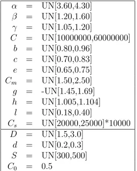
The notation used throughout the paper is as follows :
αi, βi, γi : speed, feed, depth of cut exponents for operation-tool pair i
Cm,b,c,e : specific coefficient and exponents of the machine power constraint
Cs,g,h,l : specific coefficient and exponents of the surface roughness constraint
vi : cutting speed for operation-tool pair i
fi : feed rate for operation-tool pair i
Di : diameter of the generated surface for the job i
di : depth of cut for job i
Cti : cost of tooling for operation-tool pair i
Li : length of the generated surface for the job i
Sri : maximum allowable surface roughness for the operation i
Ci : Taylor s tool life constant for operation-tool pair i
C0 : operating cost of the CNC machine ($/min)
H : maximum available horse power for all jobs pi : processing time of job i
pu
i,pli : upper and lower bounds for the processing time of job i
wi : weight of job i
ddi : due date of job i
si : starting time of job i
Ti : Tardiness of job i
Since each job has one operation, we use the same index for both operation and job. Now, we are ready to construct the mathematical model.
3.2
Mathematical Modeling
In the last part of this section we will give the mathematical formulation of the problem. However before presenting it, we will first give how lower and upper bounds of processing times, which are used in formulating the problem, can be found and second define the cost items depending on processing times of jobs in the objective function of the formulation.
3.2.1
SMOP and Lower & Upper Bounds for Processing
Times
Single Machine Operation Problem (SMOP) is the problem of determining op-timal machining conditions for an operation considering machining and tooling costs. This problem is formulated and solved optimally by Akturk and Avci [4]. The mathematical model of SMOP is given below:
Minimize C1v−1i fi−1+ C2v(αi i−1)f (βi−1) i subject to Ct0v(αi−1) i fi(βi−1) ≤ 1 i = 1 . . . N (3.1) C0 mvibfic ≤ 1 i = 1 . . . N (3.2) C0 svigfih ≤ 1 i = 1 . . . N (3.3) vi, fi > 0 (3.4) where C1 = πDiLiC0 12 C2 = πDiLidγiiCti 12Ci Ct0 = πDiLid γi i ρi 12Ci Cm0 = Cmd e i H Cs0 = Csd l i Sri
The first term in the objective function is machining cost and the second one is the tooling cost. The constraints are tool life, machine power and surface finishing constraints, respectively.
Koylu [31] showed that the surface roughness constraint in SMOP is always binding. This means that in SMOP v, f pairs on the surface roughness constraint are dominant over all other v, f points with respect to tooling and machining costs. Thus, there is only one optimal v, f pair for SMOP and there is a one to one relation between machining conditions and processing time.
CHAPTER 3. PROBLEM STATEMENT AND MODELING 21
As we stated before, our objective is minimizing the sum of total weighted tar-diness, machining, and tooling costs. SMOP contains two terms of our objective: tooling and machining. For this reason, the processing time that corresponds to the optimal solution of SMOP gives an upper bound for our problem. If we increase the processing time above that value, the sum of tooling and machining will increase and we know that tardiness cost will not decrease. Thus, there is no gain to assign a processing time to a job which is greater than the optimal solution of SMOP.
Also there is a lower bound for the processing time of job due to the power of the machine or life of a tool. It is the intersection point of surface roughness (SR) and tool life (TL) or machine power (MP) constraints. This point can be found as follows:
If the v and f values at the intersection of TL and SR constraints From SR constraint (inequality 3.3)vi = (Cs0fih)−
1
g
put it into TL constraint (inequality 3.1) C0
t(Cs0fih) 1−α g f(βi−1) i = 1 fi = (Ct0(Cs0) 1−α g )− g h(1−α)+g(β−1) = (C0 t) −h(1−α)+g(β−1)g (C0 s) α−1 h(1−α)+g(β−1) vi = (Cs0(Ct0)− hg h(1−α)+g(β−1)(C0 s) h(α−1) h(1−α)+g(β−1))−1g = (C0 t) h h(1−α)+g(β−1)(C0 s) (1−β) h(1−α)+g(β−1) (vifi)I = (Ct0) h h(1−α)+g(β−1)(C0 s) (1−β) h(1−α)+g(β−1)(C0 t)− g h(1−α)+g(β−1)(C0 s) α−1 h(1−α)+g(β−1) (vifi)I = (Ct0) h−g h(1−α)+g(β−1)(C0 s) (α−β) h(1−α)+g(β−1) (3.5)
If the vi and fi values at the intersection of TL and SR constraints
From SR constraint (inequality 3.3)vi = (Cs0fih)−
1
g
put it into MP constraint (inequality 3.2) C0
m(Cs0)− b gf cg−hb g i = 1 fi = (Cm0 ) g hb−cg(C0 s) b cg−hb vi = (Cs0(Cm0 ) hg hb−cg(C0 s) hb cg−hb)− 1 g = (C0 s) c hb−cg(C0 m) −h hb−cg (vifi)II = (Cs0) c hb−cg(C0 m) −h hb−cg(C0 m) g hb−cg(C0 s) 1 cg−hb (vifi)II = (Cs0) c−1 hb−cg(C0 m) g−h hb−cg (3.6)
We choose the minimum of the vifi values calculated by equation 3.5 and 3.6 since
the other one must be infeasible. By using the processing time equation below, we can calculate the lower bound for the processing time of a job as follows:
pi = πDiLi 12vifi (3.7) pl i = πDiLi 12min{(vifi)I, (vifi)II}
3.2.2
Cost Items of the Problem
In this section, we give the cost items included in our objective function and show that all of them can be written depending on processing time. Actually, showing this for machining and tardiness costs is trivial. However, it requires more attention for tooling cost.
• Tooling cost of job i depending on vi and fi:
T ooli(vi, fi) =
πDiLidγiiCti
12Ci
v(αi−1)
i fi(βi−1)
Since, optimal machining conditions vi and fi are on surface roughness
constraint we can write down the tooling cost depending on only processing time of job i.
From Surface Roughness constraint, we can find vi depending on fi and
using processing time equation 3.7 we can derive tooling cost that depends on processing time. C0 svigfih = 1 =⇒ vi = (Cs0(vifi)h) 1 h−g T ooli(vi, fi) = πDiLidγiiCti 12Ci v(αi−1) i f (βi−1) i = πDiLid γi i Cti 12Ci v(αi−βi) i (vifi)(βi−1) = πDiLid γi i Cti 12Ci ((C0 s(vifi)h) (αi−βi) h−g )(v ifi)(βi−1) = πDiLid γi i Cti 12Ci (Cs0)(αi−βi)h−g (vifi)h(αi−βi)h−g (vifi)(βi−1)
CHAPTER 3. PROBLEM STATEMENT AND MODELING 23 = πDiLid γi i Cti 12Ci (C0 s) (αi−βi) h−g (v ifi) h(αi−1)−g(βi−1) h−g = (πDiLi 12vifi )h(1−αi)−g(1−βi)h−g (πDiLi 12 ) hαi−gβi h−g dγi i CtiC −1 i (Cs0) (αi−βi) h−g T ooli(pi) = cai (pi)cbi where cai = µπD iLi 12 ¶hαi−gβi h−g dγi i CtiC −1 i (Cs0) (αi−βi) h−g cbi = − h(1 − αi) − g(1 − βi) h − g
The critical point here is that cai and cbi are always positive because of
possible values of the technical coefficients such that α > β > 1, h > 0 and g < 0. Thus, the tooling cost is a convex function that is negatively proportional to the processing time.
• Machining Cost of job i depending on processing time: Machi(pi) = C0pi
• The Weighted Tardiness Cost of job i depending on processing time: T ardi(si, pi) = wiMax{0, si+ pi− ddi}
After showing that the objective function of our problem can be written de-pending on just processing times, we can formulate the problem.
3.2.3
Mathematical Formulation
Now, we will give the non-linear formulation of the problem. Actually, the con-straints of the problem are not nonlinear. However the tooling cost item in the objective function adds the nonlinearity.
Minimize Total Cost =
N
X
i=1
subject to si− sj ≥ pi− (M + pi)(1 − Xij) i, j = 1 . . . N (3.8) sj − si ≥ pj− (M + pi)Xij i, j = 1 . . . N (3.9) Ti ≥ si+ pi− ddi i, j = 1 . . . N (3.10) pli ≤ pi ≤ pui i = 1 . . . N (3.11) Xij = 0 or 1 i = 1 . . . N (3.12) Ti, si ≥ 0 (3.13) pi > 0 (3.14)
The M in the formulation represents a big number. The decision variables in this formulation are pi, si, Ti, Xij. The objective function is the summation
of three cost terms defined in the previous section. The first three constraint sets are the ones that comes from total weighted tardiness problem. The next constraint set defines the lower and upper bounds for the processing times which are calculated by using the SMOP formulation developed by Akturk and Avci [4].
As we stated in the previous chapter, 1||PwiTi is NP-hard. Actually it is
a subproblem of our problem. It is the case where processing times are fixed. Thus, our problem is extremely hard to solve. To reduce the complexity in the problem and to develop efficient algorithms, as we have done in the next chapter, we formulate the problem for a given sequence. In this way, we are free from the sequencing problem, but there is still a scheduling problem. To convert the formulation above to one for a given sequence, it is enough to throw out the binary variable equation 3.12 and replace the sets of inequalities 3.8 and 3.9 with the one below:
si+ pi ≤ si+1 i = 1 . . . (N − 1) (3.15)
Solving the problem just for a sequence possibly will not produce good solu-tions, however it gives an initial point and an insight to deal with the problem.
CHAPTER 3. PROBLEM STATEMENT AND MODELING 25
3.3
Summary
In this chapter, we have given the definition and the underlying assumptions of the problem of finding machining conditions and scheduling jobs considering total weighted tardiness. We have presented that our objective is the sum of total weighted tardiness, tooling and machining costs. We showed that all of them can be formulated in the form of their own processing times of which upper and lower bounds can also be found by using the SMOP formulation. Lastly, we presented the mathematical formulations of the original problem and the problem for a given sequence.
In the following chapter, we will present the local search algorithm for the original problem and the DP-based algorithm for the subproblem.
Proposed Heuristic Algorithms
In the previous chapter, we state our problem and give the underlying assump-tions. We also present the mathematical programming formulations for the orig-inal problem and for the problem with a given sequence. Lawler [33] has showed that the single machine total weighted tardiness problem is strongly NP-hard. Actually, it is a subproblem of our problem. When we fixed the processing times in our problem, our problem reduces to 1||PwiTi. Therefore, no algorithm is
likely to be proposed to solve the problem optimally in polynomial time. Hence, it is justifiable to try heuristic approaches to solve our problem.
Weighted tardiness problem and determination of machining conditions are generally considered as separate problems and solved at different levels of factory management. Machining conditions are determined at the design and develop-ment level and the weighted tardiness problem is solved at the operational level. By considering this perspective, in this chapter, we will first present an algorithm for our problem that uses the usual sequential approach in the industry. Then, we will give our approach that solves the machining condition and the weighted tardiness problems simultaneously. In the last section, we describe in detail the DP-based heuristic that is used to solve the subproblem where the job sequence is given.
CHAPTER 4. PROPOSED HEURISTIC ALGORITHMS 27
4.1
The Sequential Algorithm
The sequential algorithm consists of two levels. In the first level machining con-ditions, which are cutting speed and feed rate of the turning machine, are deter-mined. Both cutting speed and feed rate specify the processing time of a job. By using the processing times determined in the first level, single machine to-tal weighted tardiness problem is solved in the second level. As we design the algorithm, we use the best known procedures in each level and they are as follows: 1. The machining conditions considering tooling and machining costs are found by using the SMOP, whose mathematical model is given and explained in section 3.2.1. The procedure developed by Akturk and Avci [4] solves SMOP optimally.
2. To solve 1||PwiTiproblem where the processing times are calculated in the
first level, a Problem Space Genetic Algorithm (PSGA), designed by Avci
et al. [5], is employed. This is the best published algorithm in the literature
as stated by Avci et al. for the single machine weighted tardiness problem. Although the sequential algorithm solves the subproblems in each level opti-mally or almost optiopti-mally, its drawback is obvious. The interaction between two levels is ignored. By using the flexibilities provided by a CNC machine, the due date requirement can be satisfied better or operation cost due to machining and tooling costs can be decreased. In the next section, we give an algorithm that exploits the interaction between two levels to generate better solutions.
4.2
The Proposed Simultaneous Algorithm
The proposed algorithm for our problem is a Problem Space Genetic Algorithm (PSGA) that determines the machining conditions and solve the total weighted tardiness problem simultaneously. PSGAs are basically local search algorithms.
To develop a PSGA, it is necessary to define an initial feasible solution, a base heuristic and a neighborhood structure.
The overall quality of the base heuristic affects the overall effectiveness of the problem space approach. Thus, it is very critical to use a relatively fast base heuristic which generates a relatively good solution.
The neighborhood is constructed through perturbation of the problem data and the search is performed in the space of these perturbations. A genetic al-gorithm (GA), which is based on a formalization of natural genetics, is used to search that space. Some characteristics of GAs are as follows:
• There is a coding scheme for possible solutions of the problem and these
solutions are stored as strings. Each string is called a chromosome and each variable is referred to as gene.
• An evaluation function that estimates the quality of each solution (each
string) in the set of solutions (called the population) is used.
• An initial set of solutions to the problem (the initial population) is randomly
obtained or based on prior knowledge.
• A set of genetic operations that, using the information contained in a certain
population (referred to as generation G(t)) and a set of genetic operators, creates a new population (the next generation, G(t + 1)).
• A termination condition is defined at the end of the genetic process.
There are three main genetic operators: reproduction, crossover and mutation. The reproduction (or selection) operator creates a mating pool where strings are copied from G(t) and await the action of crossover and mutation. Those strings from G(t) with higher fitness values create a large number of copies in the mating pool. The crossover operator provides a mechanism for strings to mix attributes through a random process. The mutation operator produces the occasional alteration of a bit at a certain position in a string. Each bit is a candidate for mutation and will be selected according to the mutation probability.
CHAPTER 4. PROPOSED HEURISTIC ALGORITHMS 29
In problem space search, the chromosomes represent the perturbation vectors and genes represent the perturbation amount for a single job. The original prob-lem data is perturbed and the probprob-lem with perturbed data is solved by using the base heuristic to obtain a solution. Although the heuristic is applied on the per-turbed values, the objective function is calculated with the original data values as expected. The new perturbation values are generated from the previous pop-ulation by using the genetic algorithm instead of a random generation. Asexual and sexual reproduction and mutation operators are used in generations.
In this study, sequencing priorities of jobs, which are calculated with Apparent Tardiness Cost (ATC) dispatching rule, are perturbed.
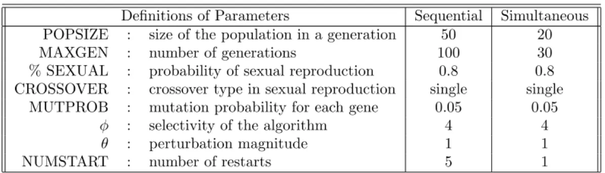
In every generation, a population of chromosomes (perturbation vectors) is created. One of the important parameters of PSGA is the POPSIZE which gives the number of perturbation vectors in a population. The perturbation magnitude
θ is the second parameter. The genes of the chromosomes can take values in a
range of (−θ, θ). The generation of initial population is done by taking random numbers in this range. Genetic algorithm operators are used in the forthcoming generations.
Fitness value shows the probability that the population member will be se-lected for breeding. The parameter φ determines the selectivity of the algorithm. The selection probability of better solutions increase as φ increases. The pop-ulation loose diversity and converge to a poppop-ulation in which all members are identical in high values of φ. However, if φ is too small, the algorithm will con-verge very slowly using excessive computation time. We will use these fitness values in asexual and sexual reproduction.
In asexual reproduction, select a member from the current population ran-domly according to selectivity (fitness) values (a random number in (0,1) is taken, and if fitness of the member is greater than this number, it is selected). This member is directly passed to the next generation. In sexual reproduction, two parents are selected in the same selectivity logic, and combined through crossover to produce an offspring which is passed to the next generation. We work on a well known single point crossover operator. In single point crossover, a point is chosen
randomly and the genes of the offspring up to that point is taken from the first parent and the following genes are copied from the second. %SEXUAL shows the percentage of sexual reproduction in the new generation. %SEXUAL·POPSIZE number of members are generated by sexual reproduction while the remaining are of asexual.
MUTPROB is the probability of mutation, and each gene has this probability to be mutated. If the gene is selected, then it is replaced by a newly generated random value taken in (−θ, θ). After mutation operation, we get the new popu-lation. Now, go to step 3 as discussed below to perturb the data with the genes of this population and calculate the objective values of the POPSIZE number of solutions produced with this data.
The whole procedure of PSGA can be summarized as follows: Step 1. Find the lower and upper bounds on processing times, pl
i and pui, for all
jobs from their SMOP formulations as stated in §3.2.1.
Step 2. Create an initial population at random from a range of (−θ, θ). Step 3. For each member (chromosome) of the population do
Step 3.1. set the current time t = 0 and number of jobs scheduled k = 0 and calculate average of averages of processing times as follows:
pavg = N X i=1 (pu i + pli)/2 N
Step 3.2. For each job i at time t, calculate the ATC priorities as follows:
ai = wi
pavgi
exp(−max(0, ddi− t − pavgi)/Kpavg)
Step 3.3. ATC priorities are normalized into interval [0,1] yielding ηi(t) as
follows, let amin(t) = miniai(t) and amax(t) = maxiai(t):
ηi(t) =
ai(t) − amin(t)
CHAPTER 4. PROPOSED HEURISTIC ALGORITHMS 31
Step 3.4. Perturb the priorities of the jobs with this member by adding the perturbation vector δi to the priorities as follows:
ηi(t) = ηi(t) + δi
Step 3.5. Select the job with the highest perturbed priority and schedule it next in the sequence. Set t = t + pavgi and k = k + 1. If there are
any unscheduled jobs, k < N , then go to step 2.1.
Step 3.6. For newly generated sequence, find the schedule by the base heuristic, which is the mathematical formulation given below or the DP-based heuristic explained in the next section, and calculate the objective function value for the given perturbation vector, denoted by
V (i).
Minimize Total Cost =
N X j=1 (wjTj + Machj(pj) + T oolj(pj)) subject to sj+ pj ≤ sj+1 j = 1 . . . (N − 1) (4.1) pl j ≤ pj ≤ puj j = 1 . . . N (4.2) sj ≥ 0 (4.3) pj > 0 (4.4) where Tj = max{0, sj+ pj− ddj}
Step 4. After finishing all members in the population, save the best and worst solutions. If the number of generations reaches the limit, then stop and report the best solution, else go to step 4 to generate a new population.
Step 5. Compute the fitness f (i) of each member as follows, Let Vmax be the
maximum objective value in the population:
fi = (Vmax− Vi) φ
P
i(Vmax− Vi)φ
Step 6. Apply crossover and mutation to get the next generation using the fitness distribution and update perturbation vectors, then go to step 2.
The algorithm above presents a single-start PSGA. It proceeds until the num-ber of generations reaches MAXGEN. However, in multi-start, after generating that much populations, the algorithm restarts itself from the first step for NUM-START times. The PSGA generates as many as the multiplication of POPSIZE, MAXGEN, and NUMSTART for each run.
4.3
The Proposed DP-based Heuristic
In this section, we present the proposed heuristic to solve the problem for a given sequence, for which we already gave the mathematical formulation in §3.2.3. This algorithm is to be used as an evaluation function (step 3.6) in the problem space genetic algorithm described in the previous section.
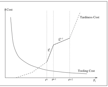
The motivation behind this algorithm was that if we can minimize the con-tribution of each job to the total cost, we can minimize the total cost. Thus we defined a contributed cost function for each job as follows:
ContCosti(pi) = T ooli(pi) + Mach(pi) + N
X
j=i
wj∆T ardj(pi) (4.5)
Each cost item in this function can be defined as the tooling cost, machining cost, and the deviation in the tardiness costs of itself and all jobs after itself depending on its own processing time. In constructing this function, we assumed that pk= plk for k = 1 . . . i − 1, since otherwise we cannot define the contributed
cost just depending on the processing time of job i because ∆T ardj, which is
the deviation in the tardiness cost of job j, is also affected from the change in processing times of those jobs. By fixing them, we define ∆T ardi over just pi.
In our algorithm, finding this contributed cost is named as Graph Generation, which corresponds to steps 2 and 3 below, since we generate a graph that shows how the contributed cost of job i changes.
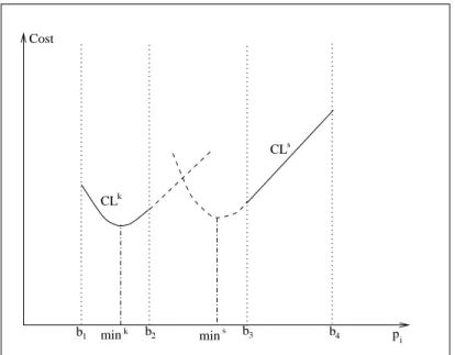
For each job, we can easily construct the function above. However we cannot directly get the processing time that minimizes it and then use them to find the final schedule. The reason is that we assumed that processing times of the
![Figure 4.3: r [k+1] − min k ≤ ∆ i < r [k+1] − min k+1](https://thumb-eu.123doks.com/thumbv2/9libnet/6007436.126541/55.918.277.690.215.556/figure-r-k-min-k-i-lt-min.webp)
![Figure 4.4: r [k] − min k ≤ ∆ i < r [k+1] − min k](https://thumb-eu.123doks.com/thumbv2/9libnet/6007436.126541/56.918.275.689.181.542/figure-r-k-min-k-i-lt-min.webp)