a dissertation submitted to
the department of industrial engineering
and the institute of engineering and science
of bilkent university
in partial fulfillment of the requirements
for the degree of
doctor of philosophy
By
Ömer Selvi
November, 2008
Asst. Prof. Dr. Ka¼gan Gökbayrak (Supervisor)
I certify that I have read this thesis and that in my opinion it is fully adequate, in scope and in quality, as a dissertation for the degree of doctor of philosophy.
Prof. Dr. M. Selim Aktürk
I certify that I have read this thesis and that in my opinion it is fully adequate, in scope and in quality, as a dissertation for the degree of doctor of philosophy.
Prof. Dr. Erdal Erel
Prof. Dr. Ömer K¬rca
I certify that I have read this thesis and that in my opinion it is fully adequate, in scope and in quality, as a dissertation for the degree of doctor of philosophy.
Assoc. Prof. Dr. Emre Alper Y¬ld¬r¬m
Approved for the Institute of Engineering and Science:
Prof. Dr. Mehmet B. Baray Director of the Institute
SERVICE TIME OPTIMIZATION OF FLOW SHOP
SYSTEMS
Ömer Selvi
Ph.D. in Industrial Engineering
Supervisor: Asst. Prof. Dr. Ka¼gan Gökbayrak November, 2008
One of the key questions that engineers face in ‡ow shop systems is the service time control, i.e., how long jobs should be processed at each machine. This is an important question because processing times can have great impacts on the cost e¢ ciency of the ‡ow shop systems. In order to meet job completion deadlines and to decrease inventory costs, one may set the service times as small as possible; however, this usually comes at the expense of reduced tool life increasing service costs. In this thesis, we study the ‡ow shop systems under such trade-o¤s. We consider the service time optimization of deterministic ‡ow shop systems process-ing identical jobs that arrive at the system at known times and are processed in the order they arrive within deadlines. The cost function to be minimized con-sists of service costs at machines and regular completion-time costs of jobs. The decision variables are the service times that are controllable within constraints.
We …rst consider the …xed service time ‡ow shop systems formed of initially controllable machines, where the service times are set only once at the start up time and cannot be altered between processes, and uncontrollable machines, where the service times are …xed and known in advance. For such systems, we formulate a non-convex and non-di¤erentiable optimization problem with a stan-dard solution procedure based on the linearization of the constraints allowing for a convex optimization problem with high memory requirements. Regardless of the cost function, we present a set of waiting and completion time characteristics in such ‡ow shop systems and employ them to derive a simpler equivalent convex optimization problem which improves solution times and alleviates the memory requirements enabling solutions for larger systems. However, the resulting sim-pli…ed convex optimization problem still needs the use of a convex optimization solver which may not be available at some of the manufacturing companies. To
decreasing service cost structure allowing us to introduce a new search algorithm much faster than the subgradient solution algorithm.
Building on the results for …xed service time ‡ow shop systems, we also con-sider the mixed line ‡ow shop systems formed of fully controllable machines, where the service times are adjustable for each process, initially controllable ma-chines, and uncontrollable machines. Similarly, we formulate a non-convex and non-di¤erentiable optimization problem for such systems and, as a standard way of solving the formulated problem, we apply the method of linearization on the constraints to present a convex optimization problem with high memory require-ments. Then, we present a set of optimal waiting characteristics in such ‡ow shop systems and employ them to derive simpler equivalent convex optimization problems. A "forward in time" algorithm is also proposed to decompose the resulting simpli…ed equivalent convex optimization problem into smaller convex optimization problems for the ‡ow shop systems formed of only fully control-lable and uncontrolcontrol-lable machines. The computational results demonstrate that the simpli…cations and the decomposition not only improve the solution times considerably but also allow us to solve larger problems by alleviating memory constraints.
Keywords: Deterministic ‡ow shop systems, Optimal control, Controllable service times, Controllable/Uncontrollable machines, Convex programming, Subgradient algorithm.
AKI¸
S T·
IP·
I ·
I¸
SL·
IK S·
ISTEMLERDE ·
I¸
SLEM SÜRELER·
I
EN·
IY·
ILEMES·
I
Ömer Selvi
Endüstri Mühendisli¼gi, Doktora
Tez Yöneticisi: Asst. Prof. Dr. Ka¼gan Gökbayrak Kas¬m, 2008
Mühendislerin ak¬¸s tipi i¸slik sistemlerde cevaplamas¬gereken en kilit sorulardan birisi i¸slem sürelerinin nas¬l denetlenece¼gidir yani i¸slerin her makinede ne kadar süre i¸slem görmesi gerekti¼gidir. Bu önemli bir sorudur çünkü i¸slem sürelerinin ak¬¸s tipi i¸slik sistemlerin maliyet verimlili¼gi üzerinde çok büyük etkileri olabilir. ·
I¸sleri son bitim zaman¬na kadar tamamlamak ve envanter maliyetlerini dü¸sürmek için i¸slem süreleri mümkün oldu¼gunca küçük tutulabilir, fakat bu yakla¸s¬m genel-likle i¸slem maliyetlerini yükselten k¬salt¬lm¬¸s tak¬m ömürlerinden do¼gan masra‡ar¬ beraberinde getirir. Biz bu tezde ak¬¸s tipi i¸slik sistemlerde bu tip ili¸skiler üzer-ine çal¬¸st¬k. Bilinen zamanlarda gelen i¸sleri geldikleri s¬rayla i¸sleyen belirlen-imci ak¬¸s tipi i¸slik sistemlerde i¸slem süreleri eniyilemesi problemini ele ald¬k. Enküçültülecek maliyet fonksiyonunu makinelerdeki i¸slem maliyetlerinden ve ku-rall¬i¸s bitim zaman¬maliyetlerinden olu¸sturduk. Bir k¬s¬t dahilinde denetlenebilir i¸slem sürelerini karar de¼gi¸skenleri olarak belirledik.
Öncelikle, ba¸slang¬çta denetlenebilir, yani i¸slem süreleri sistemin çal¬¸smaya ba¸slama an¬nda belirlenen ve i¸slemler aras¬nda bir daha de¼gi¸stirilemeyen, ve denetlenemez, yani i¸slem süreleri sabit olan ve önceden bilinen, makinelerden olu¸san sabit i¸slem süreli ak¬¸s tipi i¸slik sistemleri ele ald¬k. Bu tip sistemler için standart çözüm yöntemi yüksek bellek gereksinimli bir d¬¸sbükey eniyileme prob-lemine olanak sa¼glayan k¬s¬tlar¬n do¼grusalla¸st¬r¬lmas¬metoduna dayanan d¬¸sbükey olmayan ve türevlenemeyen bir eniyileme problemi olu¸sturduk. Maliyet fonksiy-onundan ba¼g¬ms¬z olarak, bu tip ak¬¸s tipi i¸slik sistemler için bir dizi bekleme ve i¸s bitim zaman¬özellikleri gösterdik ve bu özellikleri kullanarak çözüm sürelerini geli¸stiren ve daha büyük sistemlerin çözülmesine olanak sa¼glayacak ¸sekilde bellek gereksinimini azaltan daha basit ve denk bir d¬¸sbükey eniyileme problemi ç¬kard¬k. Ne var ki sonuçta ortaya ç¬kan basitle¸stirilmi¸s d¬¸sbükey eniyileme problemi hala
goritmas¬e¸sli¼ginde bir ba¸ska denk d¬¸sbükey eniyileme problemi önerdik. Ayr¬ca, altgradyan algoritmas¬ndan çok daha h¬zl¬ çal¬¸san yeni bir tarama algoritmas¬ geli¸stirmemize olanak sa¼glayan do¼grusal olmayan ve azalan özel bir i¸slem maliyet yap¬s¬n¬da çözümledik.
Sabit i¸slem süreli ak¬¸s tipi i¸slik sistemler için geçerli sonuçlar¬n üzerine in¸sa etmek suretiyle, bu tezde ayr¬ca tamamen denetlenebilir, yani i¸slem süreleri her i¸slem için ayr¬ ayr¬ ayarlanabilen, ba¸slang¬çta denetlenebilir ve denetlene-mez makinelerden olu¸san ak¬¸s tipi i¸slik sistemleri de ele ald¬k. Benzer ¸sekilde, bu tip sistemler için d¬¸sbükey olmayan ve türevlenemeyen bir eniyileme prob-lemi olu¸sturduk ve olu¸sturdu¼gumuz bu probleme standart çözüm yöntemi olarak, k¬s¬t do¼grusalla¸st¬rma metodu uygulamak suretiyle yüksek bellek gereksinimli bir d¬¸sbükey eniyileme problemi ortaya koyduk. Daha sonra, bu tip ak¬¸s tipi i¸slik sis-temler için bir dizi en iyi bekleme özellikleri gösterdik ve bu özellikleri kullanarak daha basit ve denk bir d¬¸sbükey eniyileme problemi ç¬kard¬k. Sadece tamamen denetlenebilir ve denetlenemez makinelerden olu¸san ak¬¸s tipi i¸slik sistemler için, sonuçta ortaya ç¬kan basitle¸stirilmi¸s d¬¸sbükey eniyileme problemini daha küçük d¬¸sbükey eniyileme problemlerine ayr¬¸st¬ran "zamanda ilerleyen" bir algoritma da önerdik. Deneysel hesaplamalar¬m¬z gösterdi ki basitle¸stirmeler ve ayr¬¸st¬rma sadece çözüm sürelerini geli¸stirmekle kalmad¬ayn¬zamanda bellek gereksinimini azaltmak suretiyle daha büyük sistemleri çözmemize olanak sa¼glad¬.
Anahtar sözcükler : Belirlenimci ak¬¸s tipi i¸slik sistemler, En iyi denetleme, Denetlenebilir i¸slem süreleri, Denetlenebilir/denetlenemez makineler, D¬¸sbükey programlama, Altgradyan algoritmas¬.
my family
I would like to sincerely thank my advisor Asst. Prof. Dr. Ka¼gan Gökbayrak for his valuable and perpetual guidance and encouragement throughout this study. His supervising with patience and interest made this thesis possible.
I gratefully acknowledge all the members of my committee who have given their time to read this manuscript and o¤ered valuable advice.
My special thanks go to my family for their encouragement and sacri…ce. This study is dedicated to them without whom it would not have been possible.
1 Introduction 1
2 Fixed Service Time Flow Shop Systems 9
2.1 Problem Formulation . . . 11
2.2 Waiting Characteristics of Fixed Service Time Flow Shop Systems 15 2.3 Simpli…ed Convex Optimization Problem . . . 26
2.4 Subgradient Descent Algorithm with Projections . . . 27
2.5 Two-Phase Search Algorithm . . . 32
2.5.1 Determining the Minimizers of fJkgNk=1 Functions . . . 35
2.5.2 Locating the Optimal Solution of JR . . . 41
2.5.3 The Algorithm . . . 48
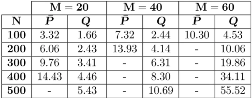
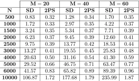
2.6 Numerical Study . . . 50
2.6.1 Veri…cation of the Waiting Characteristics . . . 50
2.6.2 Comparison of Di¤erent Solution Methodologies . . . 52
2.7 Conclusion . . . 56
3.2 Waiting Characteristics of the Optimal Sample Path . . . 64
3.2.1 Initially Controllable Portions . . . 64
3.2.2 Fully Controllable Portions . . . 72
3.3 Simpli…ed Convex Optimization Problems . . . 83
3.3.1 Flow Shop Systems Starting with Fully Controllable Portions 83 3.3.2 Flow Shop Systems Starting with Initially Controllable Por-tions . . . 85
3.4 Forward Decomposition Algorithm . . . 88
3.5 Numerical Study . . . 100
3.5.1 Veri…cation of the Optimal Waiting Characteristics . . . . 101
3.5.2 Analysis of the Replacement of Initially Controllable Ma-chines with Fully Controllable MaMa-chines . . . 103
3.5.3 Analysis of the E¤ects of the Locations of Fully Control-lable Machines . . . 104
3.5.4 Analysis of the Relative E¤ects of Service and Completion-Time Costs on the Optimal Solution . . . 106
3.5.5 Comparison of Di¤erent Solution Methodologies . . . 107
3.6 Conclusion . . . 111
4 Conclusion 113 4.1 Concluding Remarks . . . 113
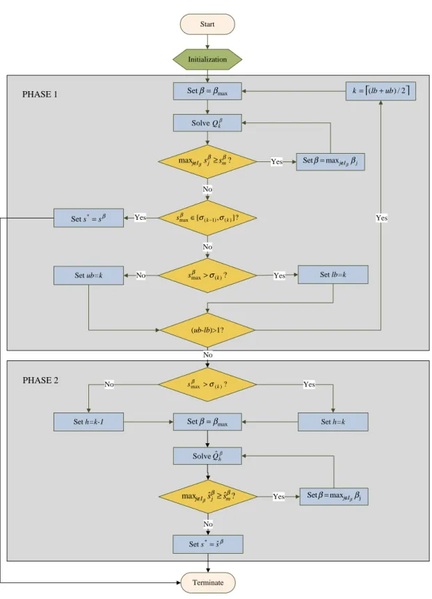
2.1 Flowchart of the Two-Phase Search Algorithm . . . 49
2.2 Evolutions of Service Times for Subgradient Descent Algorithm . 53
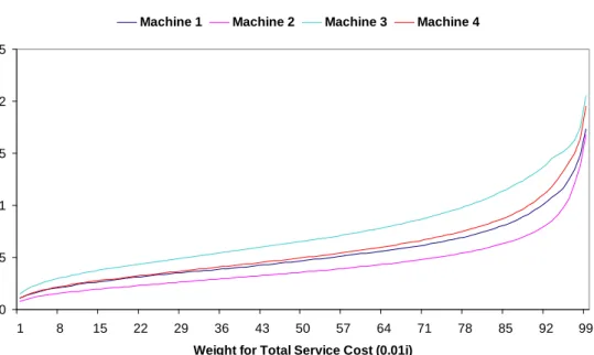
3.1 Optimal Service Times Averaged over All Jobs at Machines versus Weight of Total Service Cost . . . 107
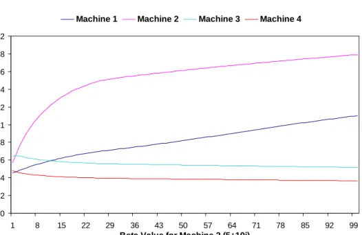
3.2 Optimal Service Times Averaged over All Jobs at Machines versus
2 value at Machine 2 . . . 108
2.1 Optimal Departure Times . . . 52
2.2 Computation Times for P and Q Formulations (in seconds) . . . . 54
2.3 Computation Times for Q Formulation and Subgradient Descent Algorithm (in seconds) . . . 55
2.4 Computation Times for Subgradient Descent and Two-Phase Search Algorithms (in seconds) . . . 55
3.1 Optimal Service Times . . . 102
3.2 Optimal Departure Times . . . 102
3.3 Optimal Costs of Di¤erent Replacement Actions for Alternative Systems . . . 103
3.4 Optimal Costs for Di¤erent Layout Con…gurations with only One Fully Controllable Machine . . . 105
3.5 Optimal Costs for Di¤erent Layout Con…gurations with Two Fully Controllable Machines . . . 105
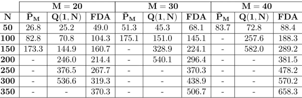
3.6 Computation Times for PM and Q(1; N ) Formulations, and
For-ward Decomposition Algorithm (in seconds) . . . 109
Introduction
Flow shop systems have been an important area of research ever since 1950’s. Since ‡ow shop systems can often be found throughout many industries, i.e., manufacturing (e.g. automobile) industry, many researchers have recognized the importance of the subject and contributed to it. One of the key questions that engineers face in ‡ow shop systems is the service time control, i.e., how long jobs should be processed at each machine. This is an important question because service times can have great impacts on the cost e¢ ciency of ‡ow shop systems.
Taylor’s tool wear equation [24] states that tool life decreases rapidly with an increase in machining speed. Increased machining speeds may also result in more frequent tool breakages. Hence, increasing machining speeds rapidly increases the frequency of tool changing which implies increased tooling costs. Moreover, tooling has also direct cost implications. Industry data suggests that tooling, as one of the major component, accounts for 25% to 30% of production cost in an automated machining environment (see [26]). In ‡exible manufacturing systems (FMSs), the initial investment in cutting tools and …xtures may reach up to 25% of the total FMS investment (see [46]). Seven to ten times more money is spent on tools, jigs, …xtures, and consumables than on capital equipment during the useful life of the machines (see [3]). The impact of tooling problems on system management should also not be underestimated: 40% to 60% of a foreman’s time is spent expediting tools and materials, 15% to 20% of scheduled production time
is missed due to unavailable tooling.
It is evident from the above discussion that, to decrease tooling costs, it is preferred to decrease machining speeds and, therefore, to increase service times as much as possible. However, longer service times mean longer ‡ow times (time required to move a job through the system, from entry on the …rst machine to completion on the last machine) of jobs. Increased ‡ow times require the antici-pation of customers’needs in terms of product variations, options, and extra …n-ished goods as well as work-in-process (WIP) inventories due to longer deliveries. Capital invested to inventories as long as they remain in the system provides no pro…t. Inventory quality also decreases as the un…nished items spend more time in the system because they are vulnerable to damages. Moreover, the ability to adapt the production structure according to the fast changing global market and to respond customer needs relies on shorter ‡ow times and lower work-in-process inventories. For instance, a manufacturing system with shorter ‡ow times elim-inates the necessity of further …nished products and WIP inventories, provides greater freedom of choice to the customer, and, therefore, becomes more com-petitive against any alternative system with longer delivery times. Many other advantages such as correcting quality problems and implementing engineering changes accompany to these due to faster responsiveness. Hence, to decrease the cost related to inventory held and customer satisfaction, which is hard to be quanti…ed, service times are tried to be reduced as much as possible.
In this thesis, we study the ‡ow shop systems under such trade-o¤s. We con-sider the service time optimization of deterministic ‡ow shop systems processing identical jobs that arrive at the system at known times and are processed within their associated deadlines. The term "identical" used for jobs implies that the operational requirements of all jobs so as to change their physical characteristics according to certain speci…cations are the same at each machine so that each machine has its own speci…c service cost function applied to all jobs processed, i.e., homogeneous (same for each job but not for each machine) service cost func-tions are employed for jobs at machines. The ‡ow shop system that we consider consists of fully controllable machines, where the service times are adjustable be-fore each process, initially controllable machines, where the service times are set
only once at the start up time and could not be altered between processes, and uncontrollable machines, where the service times are …xed and known a priori. The existing CNC (Computer Numerical Control) machine technology allows us to change the service times very quickly by just changing few lines in the CNC programming code without incurring setup times and production errors. Hence, CNC machines are good examples of fully controllable machines. As opposed to CNC machines, some traditional (non-CNC) machines are manually controlled by human operators. During mass production, it may not be feasible to alter the service times of these machines because the setup times are idle times and the manual modi…cations are prone to errors. Therefore, the service times at these traditional machines are uncontrollable or initially controllable, i.e., they are set at the start-up time and are not altered afterwards. The cost objective we consider consists of service costs at fully and initially controllable machines, which are dependent on service times, and regular completion-time costs for jobs. Motivated by the above discussion, we assume that faster services increase service costs. Slower services, on the other hand, increase the regular completion-time costs and/or leading to the violation of constraints on job completion deadlines. This trade-o¤ in setting the service times makes the problem nontrivial and we set our objective to determine the cost-minimizing service times.
The scheduling problems of the ‡ow shops are known to be NP-hard even for …xed service times (see [39]). In these problems, the objective is to …nd the best sequence of jobs to be processed at machines. Except for two-machine systems with the objective of minimizing makespan, the scheduling literature for the ‡ow shop systems is limited to heuristics and approximate solution methods. Introduction of controllable service times at machines further complicates the problem. A survey of results on the controllable service times in scheduling problems can be found in [36], [19], and [44]. In this thesis, searching for e¢ cient solution methodologies yielding true optimal solutions, we assume that jobs are processed in the order they arrive at machines, i.e., the machines operate on a non-preemptive …rst-come …rst-served policy.
The related optimal control literature, on the other hand, assumed that jobs are processed in a given sequence, and concentrated on determining the optimal
control inputs which in turn determine the optimal service times. The idea of treating scheduling problems for deterministic queues as optimal control problems on discrete event dynamic systems …rst appeared in [12] where job arrival times to a single machine system were controlled to minimize the discrepancy between job completion times and desired due dates. Following this work, service time control problems for the systems, where the job arrival times are known in ad-vance and the service times can be adjusted between processes, were considered. Pepyne and Cassandras, in [37], formulated a non-convex and non-di¤erentiable optimal control problem for a single machine system with the objective of com-pleting jobs as fast as possible with the least amount of control e¤ort and used calculus of variations techniques to obtain structural properties of the optimal solution. In [38], Pepyne and Cassandras extended their results to jobs with non-regular completion-time costs penalizing earliness and tardiness with given due dates. The task of solving these problems was simpli…ed by exploiting structural properties of the optimal sample path and it was shown that the optimal solution is unique by Cassandras et al. [7]. Further exploiting the structural properties of the optimal sample path for the single machine problem, “backward in time” and "forward in time" algorithms based on the decomposition of the original non-convex and non-di¤erentiable optimization problem into a set of smaller non-convex optimization problems with linear constraints were presented by Wardi et al. [47] and Cho et al. [10], respectively. The "forward in time" algorithm presented by Cho et al. [10] was later improved by Zhang and Cassandras [48]. In a related work, Cassandras and Mookherjee [6] studied the case of uncertainty where only some future arrival information is available within a time window of length T and introduced a receding horizon control scheme along with its several properties en-abling the use of a controller based on rough estimates of unknown future arrivals with limited loss of optimality properties. Moon and Wardi [34] considered a sin-gle machine problem where the completed jobs wait in a …nite size output bu¤er until their due dates. They presented an e¢ cient solution algorithm for this system with blocking. Mao et al. [32] removed the completion-time costs and introduced deadline constraints. Some optimal solution properties of the result-ing problem were identi…ed leadresult-ing to a highly e¢ cient solution algorithm under the assumption that a feasible solution exists. In the absence of feasible solutions
due to deadline constraints, Mao and Cassandras [29] introduced an admission control scheme in which some jobs are removed with the objective of maximizing the number of remaining jobs which are all guaranteed feasibility and, through derivation of several optimality properties, developed a computationally e¢ cient algorithm for solving the resulting admission control problem.
Flow shop systems are not the simple extensions of the single machine sys-tems. It is much more di¢ cult to solve the service time optimization problems in ‡ow shop systems for two main reasons: i) there is an M -fold (where M 2 is the number of machines in the ‡ow shop) increase in the dimensionality of the decision variables, and ii) coupling among the machines’dynamics causes the fail-ure of the structural properties exploited in single machine systems. Due to these di¢ culties, only a few works were conducted on the service time optimization problems on ‡ow shop systems in the optimal control literature. The work on service time control problems for ‡ow shop systems with identical jobs started out with Cassandras et al. [5], which derived some necessary conditions for optimality and introduced a solution technique using the Bezier approximation method for a two-machine ‡ow shop system. Recently, building on the works in [32], Mao and Cassandras [30] considered two-machine ‡ow shop systems with service costs that are decreasing on service times and derived some optimality properties that led to an iterative algorithm, which was shown to converge. The results in [30], were later extended to multi-machine ‡ow shop systems with nonidentical jobs by Mao and Cassandras [31]. To the best of our knowledge, Mao and Cassandras [31] is the only study on service time optimization of multi-machine ‡ow shop systems in the optimal control literature. Therefore, we can say that service time optimization of ‡ow shops needs further attention and we aim to contribute to the literature in that sense.
In this thesis, we consider the ‡ow shop system in Mao and Cassandras [31] with identical jobs and introduce initially controllable and uncontrollable ma-chines, and job completion-time costs. Although it seems to be a simple extension, structural properties allowing for an e¢ cient solution procedure for the system in [31], which focuses only on service costs at machines, no longer hold when we include job completion-time costs in the objective function even in the absence
of initially controllable and uncontrollable machines. Hence, the analysis changes completely. We …rst formulate an optimization problem minimizing a convex cost objective over a non-convex feasible region due to max-plus algebra used for the representation of departures of jobs from machines, which is, therefore, non-convex and non-di¤erentiable. The standard way of solving this non-convex and non-di¤erentiable problem is indeed to apply linearization on the equality constraints including max function to convexify the feasible region. However, the linearization process, which replaces each max equality constraint with two inequality constraints, doubles the number of constraints in the resulting convex formulation. Hence, the numeric solution of this convex optimization problem demands a large memory limiting the solvable system sizes due to its increased dimensionality. Hence, we search for more e¢ cient solution methodologies in terms of both solvable system sizes and solution times in this thesis.
In Chapter 2, we consider the ‡ow shop systems consisting only of initially controllable and uncontrollable machines termed …xed service time ‡ow shop sys-tems. In order to relieve the memory bottleneck for the convex formulation derived through aforementioned linearization process, we present a set of wait-ing and completion time characteristics of …xed service time ‡ow shop systems regardless of the cost objective. Mainly, we show that no waiting is observed after the slowest machine, i.e., machine with the highest service time, of the sys-tem and jobs that do not wait at the slowest machine observe no waiting in the system. Based on these results, we introduce two alternative representations for the job completion times. Employing the …rst representation, we derive a simpli-…ed equivalent convex optimization problem, which improves the solution times and enables solutions for larger systems due to less memory requirements than the convex optimization problem obtained through linearization. However, the resulting simpli…ed convex optimization problem still needs the use of a convex optimization solver which may not be available at some of the manufacturing companies. Hence, motivated by the need for a lower cost optimization tool, we employ the second representation of job completion times to introduce another equivalent convex optimization problem, which is non-di¤erentiable, along with its subgradient descent algorithm. As demonstrated by a numerical study, the
subgradient descent algorithm not only eliminates the need for convex optimiza-tion solvers but also allows for the soluoptimiza-tion of larger systems due to its much less memory requirements and improves the solution times signi…cantly. We also an-alyze a speci…c service cost structure inversely proportional to the services times. This cost structure allows us to sort the optimal service times of the machines and to introduce a new search algorithm much faster than the subgradient descent solution algorithm.
In Chapter 3, building on the results for …xed service time ‡ow shop sys-tems, we consider the ‡ow shop systems formed of fully controllable, initially controllable and uncontrollable machines termed mixed line ‡ow shop systems. Existence of fully controllable machines in the system brings new structural prop-erties leading to new solution methodologies di¤erent from the ones developed for …xed service time ‡op shop systems. Hence, we continue with a new chapter for mixed line ‡ow shops systems. To overcome the problem of limitation on solvable system sizes due to the huge memory requirements of the resulting convex opti-mization problem obtained through linearization on the max constraints, and to improve the solution times, we …rst present a set of optimal waiting character-istics of these systems. In particular, under the strict convexity assumption of service costs, we show that jobs do not wait on the optimal sample path after the …rst fully controllable machine. Employing the no-wait property, we then derive simpli…ed equivalent convex optimization problems. For the ‡ow shop systems formed of only fully controllable and uncontrollable machines, the asso-ciated simpli…ed equivalent convex optimization problem is then decomposed by a "forward in time" algorithm into smaller convex optimization problems under an additional strict convexity assumption on the job completion-time costs. As shown by a computational study, the simpli…cations and the decomposition not only improve the solution times considerably but also allow us to solve larger problems by alleviating memory constraints.
The rest of the thesis is organized as follows: In Chapter 2, we formulate a non-convex and non-di¤erentiable optimization problem for the ‡ow shop sys-tems formed of initially controllable and uncontrollable machines and obtain a convex programming formulation by the standard method of linearization. A set
of waiting and completion time characteristics of these systems regardless of the objective function is derived. These characteristics are then employed to derive a simpler equivalent convex optimization problem and another alternative equiv-alent convex optimization problem along with a subgradient descent algorithm. Finally, a new search algorithm is developed for a speci…c nonlinear decreasing service cost structure in this chapter. In Chapter 3, we formulate a non-convex and non-di¤erentiable optimization problem for the ‡ow shop systems formed of fully controllable, initially controllable, and uncontrollable machines and ob-tain a convex programming formulation by the standard method of linearization. We derive a set of optimal waiting characteristics of such systems and exploit them to derive equivalent simpli…ed convex optimization problems. A forward decomposition algorithm is also presented in this chapter to decompose the asso-ciated simpli…ed convex optimization problem into smaller convex optimization problems with linear constraints. Finally, we give concluding remarks, model extensions, and future research directions in Chapter 4.
Service Time Optimization of
Fixed Service Time Flow Shop
Systems
In this chapter, we consider deterministic ‡ow shop systems formed only of ini-tially controllable and uncontrollable machines processing identical jobs with known arrival times and deadlines. Since the service times are …xed at the start-up time and are not changed during the whole process, we de…ne these systems as …xed service time ‡ow shops. The cost function we consider consists of service costs at initially controllable machines and regular completion-time costs of jobs. Motivated by the extended Taylor’s tool-wear equation [24], we assume that faster services increase wear and tear on the tools due to increased temperatures, and may raise the need for extra supervision, increasing service costs. The losses of the product quality due to faster services are also lumped into these service costs. Slower services, on the other hand, may delay the completion times increasing the completion-time costs and/or leading to untimely job completions. We ac-knowledge this trade-o¤ and set our objective as to determine the cost-minimizing service times.
In this chapter, we formulate a non-convex and non-di¤erentiable optimization
problem and apply the standard method of linearization on the max constraints to get a convex formulation. Since, the resulting convex formulation provides solution only for small systems due to its high memory requirements, aiming to solve larger systems and to improve solution times, we …rst derive a set of waiting and completion time characteristics for such systems independent of the cost ob-jective. Basically, we show that no waiting is observed at the downstream of the machine with the highest service time and if a job does not wait at this machine, it also observes no waiting in the system. Then, we exploit these waiting charac-teristics to derive an alternative representation of job completion times allowing us to present a simpler equivalent convex optimization problem. However, even though the resulting convex problem formulation improves the solution times and enables solutions for larger systems, it still needs the use of a solver which may not be available at some manufacturing companies. Hence, further exploiting the waiting and completion time characteristics, we come up with another alterna-tive representation of job completion times and employ it to introduce another equivalent convex optimization problem, which is non-di¤erentiable. A subgra-dient descent algorithm is also developed for solving this optimization problem. This algorithm eliminates the need for a solver and has considerably low memory requirements; therefore, it allows us to solve optimization problems of even larger systems in much shorter times. We also analyze a special case where the ser-vice costs at machines are nonlinear decreasing functions of serser-vice times. This cost structure allows us to sort the optimal service times of machines. First, we de…ne di¤erentiable subproblems that can be solved easily. Employing these subproblems, we then introduce a two-phase search algorithm that converges in a …nite number of steps. Through improving the solution times drastically, this new search algorithm eliminates the need for the subgradient descent solution algorithm whose performance, as a drawback, is highly a¤ected by the selection of its termination tolerance and step sizes at each iteration.
The rest of the chapter is organized as follows: We formulate a non-convex and non-di¤erentiable optimization problem and apply the linearization method yield-ing a convex optimization problem in Section 2.1. In Section 2.2, regardless of the objective function, we derive a set of waiting and completion time characteristics
for …xed service time ‡ow shop systems. Employing the waiting and completion time characteristics in …xed service time ‡ow shop systems derived in Section 2.2, a simpler equivalent convex optimization problem is introduced in Section 2.3. In Section 2.4, an alternative equivalent convex optimization problem is presented along with a subgradient descent algorithm with projections. For a special type service cost structure inversely proportional to the service times, we de…ne dif-ferentiable subproblems and present a two-phase search algorithm in Section 2.5. Section 2.6 presents a numerical example to illustrate the waiting and comple-tion time characteristics derived in Seccomple-tion 2.2 under optimal service times. In this section, we also compare the performances of the proposed methodologies in terms of the solution times and the solvable system sizes through a computational study. Finally, Section 2.7 concludes the chapter.
2.1
Problem Formulation
The notation used throughout the chapter is as follows:
Decision Variables:
xi;j : departure time of job i from machine j.
sj : service time at machine j.
Parameters:
M : number of machines in the system. N : number of jobs that arrive at the system.
ai : arrival time of job i.
di : deadline for the completion of job i.
Sj : lower bound for the service time at machine j. j(sj) : total service cost over all jobs at machine j. i(xi;M) : completion-time cost for job i.
We consider a sequence of N identical jobs, denoted by fCig N
i=1, arriving at an
M-machine ‡ow shop system at known times 0 a1 a2 ::: aN. Machines
process one job at a time on a …rst-come-…rst-served (FIFO) non-preemptive basis (i.e. a job in service can not be interrupted until its service completion). The bu¤ers in front of the machines are assumed to be of in…nite sizes.
Without loss of generality, uncontrollable machines can be treated as if they are initially controllable machines. Hence, to keep the notation simple and to make the rest of the chapter more readable, we acknowledge the reader that we study the ‡ow shop systems consisting only of initially controllable machines whose results are applicable to ‡ow shop systems including also uncontrollable machines.
We de…ne a temporal state xi;j that keeps the departure time information of
job Ci from machine j. The relationships between the temporal states are given
by the following max-plus equations (see [4]):
xi;j = max(xi;j 1; xi 1;j) + sj; (2.1)
xi;0 = ai, x0;j = 1 (2.2)
for i = 1; :::; N and j = 1; :::; M , where the service time at machine j 2 f1; :::; Mg is denoted by sj. Note that the same service time sj is applied to all jobs at
machine j. The deadlines fdigNi=1 are imposed to jobs fCigNi=1 so that
xi;M di: (2.3)
The discrete-event optimal control problem, denoted by P , is the determina-tion of the optimal service times:
P : min sj Sj j=1;:::;M ( J = M X j=1 j(sj) + N X i=1 i(xi;M) ) (2.4)
subject to (2.1)-(2.3) for i = 1; :::; N and j = 1; :::; M . In this formulation, j
completion-time cost for job Ci. The minimum service time required at machine
j, a physical constraint, is denoted by Sj.
Due to the existence of lower bounds on the service times of machines, i.e., sj Sj for all j = 1; :::; M , the system can not guarantee that all jobs meet
their associated deadlines, that is, the optimization problem P in (2.4) may be infeasible. In this thesis, we will study the feasible case. We can handle the infeasible case by introducing an admission control mechanism through which some jobs are selected and removed so that the system becomes feasible while minimizing the number of such jobs as described for the single machine case in [29]. However, we will not consider the job admission problem here.
The following assumptions are necessary to make the problem somewhat more tractable while preserving the originality of the problem.
Assumption 2.1 : j( ), for j = 1; :::; M , is monotonically decreasing and
con-vex.
Assumption 2.2 : i( ), for i = 1; :::; N , is monotonically increasing and
con-vex.
These assumptions indicate that longer services will decrease the service costs while increasing the departure times, hence, the completion-time costs.
Due to the max function in (2.1), the optimization problem P in (2.4) is non-convex and non-di¤erentiable. A standard method for solving the optimization problem P is to replace (2.1) with two linear inequalities and to employ (2.2) for the …rst job. Since, by Assumptions 2.1 and 2.2, both costs are convex, we arrive at the following convex optimization problem:
P : min sj Sj xi;j i=1;:::;N j=1;:::;M ( J = M X j=1 j(sj) + N X i=1 i(xi;M) ) (2.5)
subject to x1;1 = a1+ s1 (2.6) x1;j = a1+ j X k=1 sk (2.7) xi;1 ai+ s1 (2.8) xi;1 xi 1;1+ s1 (2.9) xi;j xi;j 1+ sj (2.10) xi;j xi 1;j+ sj (2.11) x1;M d1 (2.12) xi;M di (2.13)
for all i = 2; :::; N and j = 2; ::; M . There are (N + 1)M variables, M equality and 2(N 1)M + N inequality constraints in this formulation excluding the M boundary value constraints on the service times.
The optimization problem P is over a larger feasible set than the optimization problem P ; therefore its optimal cost J is upper bounded by the optimal cost of P denoted by J , i.e., J J . However, it can easily be veri…ed that an optimal service time vector s for P is also an optimal solution for P with J = J . Hence, the optimal solution for the optimization problem P can be determined by solving the convex optimization problem P .
In the next section, independent of the cost structure, we derive a set of waiting and completion time characteristics of the ‡ow shop systems with …xed service times. These waiting and completion time characteristics will then allow us to present alternative equivalent convex optimization problems.
2.2
Waiting Characteristics of Fixed Service
Time Flow Shop Systems
In …xed service time ‡ow shop systems, each machine j performs some service of duration sj. Based on these service times, we de…ne the following:
De…nition 2.1 Machine u is a local bottleneck if its service time exceeds the service times of all upstream machines, i.e., su > maxj=0;:::;u 1sj where s0 is
de…ned to be zero.
Since the …rst machine is a local bottleneck, there is at least one local bottle-neck in each …xed service time ‡ow shop system.
De…nition 2.2 A contiguous set of machines fu; :::; vg form a ‡ushing portion if
1. Machine u is a local bottleneck, i.e., su > maxj=0;:::;u 1sj;
2. There are no local bottlenecks in machines fu + 1; :::; vg, i.e., su
maxj=u+1;:::;vsj;
3. If v < M , then machine (v + 1) is a local bottleneck, i.e., su < sv+1.
Each local bottleneck machine starts a ‡ushing portion, and the last ‡ushing portion is ended by machine M .
The following lemma establishes that jobs may wait at only the local bottle-neck machines.
Lemma 2.1 No waiting is observed in a ‡ushing portion after its local bottleneck machine.
Proof. (By induction) Let us consider some ‡ushing portion formed of machines fu; :::; vg. Since the …rst job does not wait at any machine, we have the basis for the induction. Now, let us assume that jobs Cr, r = 1; :::; i 1 do not wait at
machines fu + 1; :::; vg, i.e.,
xr;j xr 1;j+1 (2.14)
holds for all j = u; :::; v 1. From (2.1), we have
xi;u = max (xi;u 1; xi 1;u) + su
xi 1;u+ su (2.15)
and from the induction assumption (2.14), job Ci 1 does not wait at machine
(u + 1); therefore
xi 1;u+1 = xi 1;u + su+1: (2.16)
Since machine (u+1) resides in the ‡ushing portion started by the local bottleneck machine u, su su+1 by de…nition; hence, from (2.15) and (2.16), we get
xi;u xi 1;u+1;
i.e., job Ci does not wait at machine (u + 1). Next, in addition to (2.14), let us
assume that job Ci does not wait at machines fu + 1; :::; jg where j < v, i.e.,
xi;k xi 1;k+1 (2.17)
holds for all k = u; :::; j 1. From the induction assumptions (2.14) and (2.17), we can write xi 1;j+1 = xi 1;u+ j+1 X l=u+1 sl (2.18)
and xi;j = xi;u+ j X l=u+1 sl
= max (xi;u 1; xi 1;u) + su+ j X l=u+1 sl xi 1;u+ j X l=u sl: (2.19)
Since su sj+1 by de…nition, from (2.18) and (2.19), we have
xi;j xi 1;j+1 (2.20)
indicating that job Ci does not wait at machine (j + 1), therefore, concluding the
induction proof.
The next lemma suggests that, given the waiting status of a job at a local bottleneck machine, we may deduce its waiting status at a downstream or an upstream local bottleneck machine.
Lemma 2.2 If job Ci waits for service at some local bottleneck, then it will wait
for service at all downstream local bottlenecks.
Proof. We consider two consecutive local bottleneck machines u and (v + 1), and assume that job Ci waits at machine u, so we have
xi;u 1 < xi 1;u: (2.21)
If these two local bottleneck machines are adjacent, i.e., if v = u then, from (2.1) and (2.21), we have
xi;v = xi 1;u + su (2.22)
and
Since su < sv+1 by de…nition, from (2.22) and (2.23), we get xi;v < xi 1;v+1, i.e.,
job Ci waits at machine (v + 1).
If, on the other hand, these two local bottlenecks are not adjacent, i.e., v > u then, from (2.1), (2.21), and by Lemma 2.1, we have
xi;v = xi;u+ v
X
j=u+1
sj
= max (xi;u 1; xi 1;u) + su+ v X j=u+1 sj = xi 1;u+ su+ v X j=u+1 sj (2.24) and xi 1;v+1 = max (xi 1;v; xi 2;v+1) + sv+1 xi 1;v+ sv+1 xi 1;u+ v X j=u+1 sj + sv+1: (2.25)
Since su < sv+1 by de…nition, from (2.24) and (2.25), we get xi;v < xi 1;v+1, i.e.,
job Ci waits at machine (v + 1).
The result extends iteratively to all downstream local bottleneck machines concluding the proof.
As it turns out, waiting is observed only at the local bottleneck machines. Given the arrival times of the jobs and the service time of some local bottleneck machine u, we can determine which jobs wait at this machine. Let us de…ne the average interarrival time between jobs Ck and Cl, where k > l as
l
k =
ak al
The minimum of the average interarrival times for job Ck is, then, de…ned as k = 8 < : 1; k = 1 min l=1;:::;k 1 l k; k > 1: (2.27)
The following lemma allows us to determine whether a job waits or not at some local bottleneck machine u.
Lemma 2.3 A job Ck waits for service at the local bottleneck machine u if and
only if k< su.
Proof. (Necessity) Let us assume that Ck does not wait at the local bottleneck
machine u. According to Lemmas 2.1 and 2.2, no waiting is observed by the job at the upstream machines; therefore we have
xk;u = ak+ u
X
j=1
sj: (2.28)
For previous jobs fCigk 1i=1, we can write
xi;u ai+ u
X
j=1
sj: (2.29)
Hence, from (2.28) and (2.29), we get
xk;u xi;u ak ai (2.30)
for all i = 1; :::; k 1. Since the departure times (from machine u) of two consec-utive jobs are at least su apart, we can write
xk;u xi;u (k i)su (2.31)
for all i = 1; :::; k 1. From (2.26), (2.30), and (2.31), we have
i
for all i = 1; :::; k 1, resulting in, from (2.27),
k su:
(Su¢ ciency) Let us assume that job Ck waits at machine u. Then, we have
xk;u > ak+ u
X
j=1
sj: (2.32)
Let Ci be the last job in fC1; :::; Ck 1g that does not wait at machine u (since job
C1 does not wait at any machine, existence of such a job is guaranteed.) Then,
according to Lemmas 2.1 and 2.2, Ci does not wait at any upstream machine, so
we can write
xk;u = xi;u+ (k i)su
= ai+ u
X
j=1
sj + (k i)su: (2.33)
From (2.26), (2.32), and (2.33), we get
i k< su
resulting in, from (2.27),
k < su:
We describe the waiting characteristics of jobs at local bottleneck machines by block structures.
De…nition 2.3 A contiguous set of jobs fCigni=k is said to form a block at a
local bottleneck machine u if
1) Jobs Ck and Cn+1 (if exists) do not wait at machine u, i.e., xk;u 1 xk 1;u
2) Jobs fCigni=k+1 wait at machine u, i.e., xi;u 1 < xi 1;u for i = k + 1; :::; n.
For some local bottleneck machine u, each block starts with a non-waiting job k and continues with waiting jobs fCigni=k+1with departure times
xi;u = xk;u+ (i k)su: (2.34)
De…nition 2.4 A partition of jobs into blocks is called a block structure.
For any given service time su, by modifying the arrival times, we can generate
2N di¤erent block structures at a local bottleneck machine u. If the arrival times
are given, however, by modifying the service time su, we can generate at most N
di¤erent block structures. The next lemma establishes this upper bound on the number of di¤erent block structures at a local bottleneck machine.
Lemma 2.4 There are at most N di¤erent block structures at any local bottleneck machine u.
Proof. From Lemma 2.3, a job Ci starts a block at a local bottleneck machine
u i¤ i su. Reindexing i’s as
(1) (2) ::: (N );
each interval ( (k 1); (k)]; where (0) = 0, de…nes a block structure: If su 2
( (k 1); (k)], then all jobs in the set fCi : i (k)g start blocks at machine u
while others do not. Since there are at most N such intervals, there are at most N di¤erent block structures.
According to Lemma 2.3, one could evaluate k values for all jobs Ck and
compare them to the service time of the local bottleneck machine to determine the block structure. The following lemma, however, presents a computationally simpler way to determine the block structure, which is implemented in the sub-gradient algorithm developed in Section 2.4.
Lemma 2.5 If jobs fCigni=k form a block at machine u, then,
k i < su
is satis…ed for all i = k + 1; :::; n.
Proof. (By Induction) Since Ck starts the block, we know by de…nition that it
does not wait at machine u. Hence, by Lemma 2.3, we have k su, i.e., for all
l < k, we can write
l
k =
ak al
k l su: (2.35)
In order to show the basis step by a contradiction, we assume that
k
k+1 = ak+1 ak su: (2.36)
From (2.35) and (2.36), we get for all l < k
l k+1 = ak+1 al k + 1 l = (ak+1 ak) + (ak al) k + 1 l su+ (k l)su k + 1 l = su
resulting in k+1 su, which contradicts, by Lemma 2.3, that job Ck+1waits.
In order to show the induction step again by contradiction, we assume that
k
i < su (2.37)
for i = k + 1; :::; t 1, where t n and
k
From (2.35) and (2.38), we have l t = at al t l = (at ak) + (ak al) t l (t k)su+ (k l)su t l = su (2.39)
for all l = 1; :::; k 1. Moreover, from (2.37) and (2.38), we have
i t = at ai t i = (at ak) (ai ak) t i (t k)su (i k)su t i = su (2.40)
for all i = k + 1; :::; t 1. Hence, from (2.27), (2.39), and (2.40), we have t su,
which contradicts, by Lemma 2.3, that job Ct waits.
Starting with the …rst job C1, which starts the …rst block, this lemma can
be iteratively applied to determine the block structure at any local bottleneck machine. For this task, all we need are the arrival times of the jobs and the service time of the local bottleneck machine.
Next, we de…ne the most downstream local bottleneck machine of the ‡ow shop system as the global bottleneck, and derive the completion times of jobs.
De…nition 2.5 The local bottleneck machine m with the highest service time sm = maxj=1;:::;Msj is the global bottleneck.
There can be no local bottleneck machine downstream to a global bottleneck machine; therefore, by Lemma 2.1, no waiting is observed after the global bot-tleneck machine. Hence, the completion times can be determined as presented in the next lemma.
Lemma 2.6 The completion time of job Ci is given by
xi;M = max ai+ M X j=1 sj; xi 1;M + sm ! ; (2.41)
where x0;M = 1 and sm = maxj=1;:::;Msj is the service time of the global
bottleneck machine.
Proof. From (2.1), the departure time of job Ci from the global bottleneck
machine m is given as
xi;m = max (xi;m 1; xi 1;m) + sm: (2.42)
If job Ci does not wait at the global bottleneck machine m, i.e., if xi;m 1 xi 1;m,
by Lemma 2.2, it also does not wait at any upstream machine; therefore, we have
xi;m 1 = ai+ m 1X
j=1
sj xi 1;m: (2.43)
Hence, from (2.42) and (2.43), we get
xi;m= max ai+ m X j=1 sj; xi 1;m + sm ! : (2.44)
Since no waiting is observed after the global bottleneck machine m, from (2.44), we can write the completion time of the job Ci as
xi;M = ( xi;m; if m = M xi;m+PMj=m+1sj; if m < M = max ai+ M X j=1 sj; xi 1;M + sm ! :
Alternatively, based on the block structure at the global bottleneck machine, the completion times can also be determined as presented in the next lemma.
Then, the completion times of these jobs are given as xi;M = ak+ (i k)sm+ M X j=1 sj (2.45) for i = k; :::; n.
Proof. Machines fm; :::; Mg form the last ‡ushing portion of the system. By Lemma 2.1, jobs do not wait after the global bottleneck machine m,; hence the completion times of the jobs fCigni=k can be written as
xi;M = xi;m+ M
X
j=m+1
sj (2.46)
for i = k; :::; n. From Lemma 2.2, since Ck does not wait at the global bottleneck
machine m, it observes no waiting at the upstream machines. Hence, we can write xk;m = ak+ m X j=1 sj: (2.47)
For jobs fCigni=k+1 that wait at the global bottleneck machine m, we have
xi;m = xk;m+ (i k)sm: (2.48)
Hence, from (2.46), (2.47), and (2.48), the completion times of the jobs fCigni=k
are given as xi;M = ak+ (i k)sm+ M X j=1 sj:
In the next section, we employ the characteristics from this section to derive a simpler convex optimization problem formulation.
2.3
Simpli…ed Convex Optimization Problem
The result of Lemma 2.6 allows us to replace (2.1) and (2.2) in the optimization problem P by (2.41) resulting with the formulation
P : min sj Sj j=1;:::;M ( J = M X j=1 j(sj) + N X i=1 i(xi;M) ) (2.49) subject to x1;M = a1+ M X k=1 sk (2.50)
xi;M = max xi 1;M + max
j=1;:::;Msj; ai+ M X k=1 sk ! (2.51) x1;M d1 (2.52) xi;M di (2.53) for i = 2; :::; N .
Similarly, by linearizing the max functions in (2.51), we get the convex opti-mization problem Q given as
Q : min sj Sj xi;M i=1;:::;N j=1;:::;M ( JQ = M X j=1 j(sj) + N X i=1 i(xi;M) ) (2.54) subject to x1;M = a1+ M X k=1 sk (2.55) xi;M ai+ M X k=1 sk (2.56)
xi;M xi 1;M + sj (2.57)
x1;M d1 (2.58)
xi;M di (2.59)
for all i = 2; :::; N and j = 1; :::; M . In this formulation there are (N + M ) variables, one equality and (N 1)(M + 1) + N inequality constraints excluding the M boundary value constraints on the service times. Therefore, compared to the convex optimization problem P given in (2.5), improvements in solution times and memory requirements are expected.
Similar to the problem P , the convex optimization problem Q has a larger feasible set compared to the original optimization problem P . However, it can easily be veri…ed that the optimal solution for Q is formed of the optimal service times for P and the corresponding job completion times resulting from applying the optimal service times of P evaluated through (2.50) and (2.51). Hence, solving the convex optimization problem Q always yields an optimal solution for the optimization problem P .
Next, we further exploit the waiting and completion time characteristics de-rived in Section 2.2 to derive a minmax problem and present a subgradient descent algorithm with projections as its solution methodology.
2.4
Subgradient Descent Algorithm with
Pro-jections
In this section, we consider the ‡ow shop systems with no job completion dead-lines, i.e., we set di = 1 for i = 1; :::; N. The relaxation of deadlines on job
completion times will allow us to derive an alternative unconstrained equivalent convex optimization problem along with an e¢ cient subgradient descent algo-rithm as its solution methodology.
Let us employ Lemma 2.7 to rewrite the optimization problem P as ^ P : min sj Sj j=1;:::;M 8 < :J (s) = M X j=1 j(sj) + B(s) X b=1 nb(s) X i=kb(s) i akb(s)+ stotal+ (i kb(s))smax 9 = ;; (2.60) where, given the service times s, smax = maxj=1;:::;Msj is the service time of the
global bottleneck machine, stotal =
PM
j=1sj is the total service time, B(s) is the
number of blocks at the global bottleneck machine, kb(s)and nb(s)are the indices
of the …rst and the last jobs of the bth block, respectively.
Let Jl(s) = M X j=1 j(sj) + Bl X b=1 nb l X i=kb l i xli;M (2.61)
be a cost function, where Bl is the number of blocks, klb and nbl are the indices of
the …rst and the last jobs, respectively, of the bth block at some global bottleneck whose service time falls in the interval ( (l 1); (l)], and xli;M is the completion
time of job Ci given, by Lemma 2.7, as
xli;M = akb
l + stotal+ (i k
b l)smax:
Note that, by Assumptions 2.1 and 2.2, Jl is continuous and convex in the service
times. By Lemma 2.4, there are at most N di¤erent block structures at the global bottleneck; hence we have at most N di¤erent cost functions of this form.
If smax falls in the interval ( (l 1); (l)], then we have J (s) = Jl(s). In other
words, the formulation of J (s) di¤ers from interval to interval. The next lemma shows that J (s) can be written as the maximum of all these functions, yielding a minmax optimization problem.
Lemma 2.8 The cost function Jl(s) exceeds all other cost functions, i.e., Jl(s) =
maxt2f1;:::;NgJt(s), when smax2 ( (l 1); (l)].
Proof. Let us take an arbitrary job Ci, where i 2 f1; :::; Ng, and let job Ckl
the global bottleneck machine’s service time falls in the interval ( (l 1); (l)], i.e.,
when smax 2 ( (l 1); (l)]. The completion time in this case is given by Lemma
2.7 as
xli;M = akl+ stotal+ (i kl)smax: (2.62)
Let us also take an arbitrary block structure corresponding to some interval ( (t 1); (t)], and let Ckt start the block at the global bottleneck machine that
job Ci resides in. Similarly, by Lemma 2.7, the completion time of job Ci for this
block structure is given as
xti;M = akt + stotal+ (i kt)smax: (2.63)
Now, assume that smax2 ( (l 1); (l)]. We would like to compare Jl(s) and Jt(s)
under this assumption.
From (2.62) and (2.63), the completion times satisfy
xli;M xti;M = (akl akt) + (kt kl)smax: (2.64)
There are three cases to consider:
Case 1: For t = l, from (2.64), we have xli;M = xti;M.
Case 2: For t < l, i.e., for (t) < (l), by Lemma 2.3, kt kl because
decreasing the service time of the global bottleneck has the e¤ect of separating blocks into smaller blocks. If kt = kl, then from (2.64), xli;M = xti;M. If, on the
other hand, kt > kl, then job Ckt is in the block started by job Ckl, which leads
to kl
kt < smax by Lemma 2.5. Therefore, we have, from (2.26) and (2.64), that
xli;M xti;M = (kt kl) smax
(akt akl)
(kt kl)
= (kt kl)[smax kklt] 0:
Case 3: For t > l, i.e., for (t) > (l), by Lemma 2.3, kt kl because
blocks into larger blocks. If kt = kl, then from (2.64), xli;M = xti;M. If, on the
other hand, kt < kl, then since kl smax by Lemma 2.3, we have, from (2.26),
(2.27), and (2.64), that
xli;M xti;M = (kt kl) smax
(akl akt)
(kl kt)
= (kl kt)[ kktl smax]
(kl kt)[ kl smax] 0:
Hence, from all three cases, xl
i;M xti;M, when smax 2 ( (l 1); (l)]. By
Assump-tion 2.2, i is monotonically increasing; therefore, from (2.45) and (2.61),
Jl(s) Jt(s) = N X i=1 i(x l i;M) i(x t i;M) 0:
Since t N is arbitrary, the result follows.
Hence, by Lemma 2.8, we can write the optimization problem as
R : min sj Sj j=1;:::;M n JR(s) = max l Jl(s) o ; (2.65)
where Jl is the convex and continuous cost function corresponding to the interval
( (l 1); (l)]. Being the maximum of convex and continuous functions, JR is a
convex and continuous function of the service times.
According to Lemma 2.8, when the global bottleneck machine’s service time smax falls in an interval ( (l 1); (l)] for some l N, the cost is JR = Jl(s).
Therefore, for this case, the sensitivities of JR to service times (at di¤erentiable
points) can be written as
@JR @sj = 8 < : 0 j(sj) + PBl b=1 Pnb l i=kb l 0 i xli;M ; sj < smax 0 j(smax) + PBl b=1 Pnbl i=kb l 0
i xli;M (1 + i klb) ; (l)> sj > maxi6=jsi
(2.66) for j = 1; :::; M . Note that when sj = (l), i.e., when the block structure at the
there are other machines with the maximum service time, non-di¤erentiability is observed. For these points, we de…ne the left derivatives as
@JR @sj = 8 < : 0 j(smax) +PBb=1l P nb l i=kb l 0
i xli;M ; sj = maxi6=jsi 0 j( (l)) +PBb=1l P nb l i=kb l 0
i xli;M (1 + i klb) ; (l) = sj > maxi6=jsi
(2.67) for j = 1; :::; M .
Since JRis continuous and convex, yet not everywhere di¤erentiable, we de…ne
the subgradients as the left derivative vector with components
j =
@JR
@sj
for all j = 1; :::; M . The subgradient directions drive the following descent algo-rithm with projections, which runs until the stopping condition determined by an termination tolerance and a d distance metric is satis…ed:
Algorithm 2.1 Step 0: Start with an arbitrary initial solution s0 = (s0
1; :::; s0M).
Repeat for k = 1; 2; :::
Step 1: Determine the global bottleneck machine m = minfv : sk 1
v =
maxj=1;:::;Msk 1j g.
Step 2: Determine the block structure at the global bottleneck machine m em-ploying Lemma 2.5.
Step 3: Determine k 1j for all j = 1; :::; M .
Step 4: Update solution
sk = sk 1 k k 1 : (2.68)
In (2.68), step sizes f kg1k=1 satisfy the standard conditions 1 X k=1 2 k <1; 1 X k=1 k =1
and denotes the projection mapping onto the feasible solutions set f(s1; :::; sM) : s1 S1; :::; sM SMg. Subgradient descent algorithms with
pro-jections are known to converge to the optimal solution (see, e.g. in [2].) The computational complexity per iteration is given as O(max(M; N )), i.e., the com-putational complexity per iteration is linear in both M and N .
In the next section, we build on the results from this section and analyze the special case where the lower bounds for the services times are set to zero and the service costs are inversely proportional to the service times.
2.5
Two-Phase Search Algorithm
Most of the studies in the literature assumed the service costs to be decreasing lin-ear functions of service times. This linlin-earity assumption, however, fails to re‡ect the law of diminishing marginal returns: productivity increases at a decreasing rate with the amount of resource employed. Therefore, in this section, to assure the law of diminishing marginal returns, we employ the service cost function j( )
on machine j de…ned as
j(sj) = j
sj ; (2.69)
where j is a positive parameter, sj is the service time at machine j, and is a
positive constant. This cost structure was shown to correspond to many industrial operations in [33].
Note that the service cost function given in (2.69) is strictly convex. Hence, to make the analyses more general, including this nice property, we modify the Assumption 2.1 in the following form:
monotonically decreasing and strictly convex.
In addition to the job completion deadline constraints, we relax the lower bounds on service times, i.e. , sj 0 (Sj = 0) for j = 1; :::; M , and recall the
convex optimization formulation R in (2.65) as
R : min sj 0 j=1;:::;M JR(s) = max k=1;:::;NfJk(s)g ; (2.70) where Jk(s) is given in (2.61).
Let us de…ne ri(k), the index of the job that starts the block in which job Ci
resides for the kth block structure, as
ri(k) = max j : j (k); j i (2.71)
for all i = 1; :::; N and k = 1; :::; N . Then, the completion time of job Ci for the
kth block structure yk
i(s) can be de…ned as
yik(s) = ari(k)+ stotal+ (i ri(k)) smax (2.72)
for all i = 1; :::; N where smax = maxj=1;:::;Msj and stotal =
PM
j=1sj. As an
alternative representation in (2.61), we employ (2.72) and rewrite Jk(s) as
Jk(s) = M X j=1 j(sj) + N X i=1 i yki(s) : (2.73)
Since JR(s)is continuous, it follows from (2.70) and Lemma 2.8 that JR(s) = Jk(s)
when smax2 [ (k 1); (k)].
Another important property of the cost functions fJkgNk=1 is strict convexity,
which is presented in the next theorem.
Theorem 2.1 The cost function Jk(s), for k = 1; :::; N , is strictly convex on the
Proof. Let us de…ne two distinct feasible solutions s1 and s2 such that
sl = (sl1; :::; slM)
for l = 1; 2. For some 2 (0; 1), let s3 be
s3 = s1+ (1 )s2: (2.74)
To have strict convexity, it su¢ ces to show that the strict inequality
Jk(s1) + (1 )Jk(s2) > Jk s1+ (1 )s2 = Jk(s3) (2.75)
holds.
Due to strict convexity of j( )by Assumption 2.3, we have
M X j=1 j(s1j) + (1 ) j(s2j) > M X j=1 j s1j + (1 )s 2 j = M X j=1 j(s3j): (2.76) From (2.74), we have
s3max s1max+ (1 )s2max; s3total = s1total+ (1 )s2total:
Therefore, we obtain yik(s1) + (1 )yik(s2) = ari(k)+ s 1 total+ (1 )s 2 total + (i ri(k)) s1max+ (1 )s2max ari(k)+ s 3 total+ (i ri(k)) s3max= y k i(s 3):(2.77)
Since i is monotonically increasing and convex, we have from (2.77) that
i y k i(s 1) + (1 ) i y k i(s 2) i y k i(s 1) + (1 )yk i(s 2) i y k i(s 3)
for all i = 1; :::; N . Hence, we have N X i=1 i y k i(s 1) + (1 ) i y k i(s 2) N X i=1 i y k i(s 3) : (2.78)
The inequalities (2.76) and (2.78) imply (2.75) resulting with that Jkis strictly
convex.
Since JRis the maximum of Jk’s, the following corollary follows from Theorem
2.1:
Corollary 2.1 JR(s) is strictly convex function on the service times vector s =
(s1; :::; sM).
Since fJkgNk=1 and JR are strictly convex, they have unique minimizers. The
search algorithm that we construct requires us to determine the minimizers of fJkgNk=1. Hence, we …rst develop an e¢ cient method to determine these unique
minimizers.
2.5.1
Determining the Minimizers of
fJ
kg
Nk=1Functions
Let fskgNk=1 be the unique minimizers of fJkgNk=1. Note that, by Assumption 2.2,
we have
lim
sj!1 i
yki(s) =1 (2.79)
for all j = 1; :::; M ; therefore, the unique minimizers are …nite. Moreover, since the cost structure in (2.69) satis…es
lim sj!0+ j(sj) = lim sj!0+ j sj =1 (2.80)
for all j = 1; :::; M , then sk j > 0.
In the next lemma, we state that there exists an ordering among the optimal service times sk
Lemma 2.9 For any two machines u and v, if u v then sku skv.
Proof. For a contradiction, let us assume that while u v, the optimal service times satisfy
sku < skv (2.81) and de…ne the perturbed service times sj for j = 1; :::; M as
sj = 8 > > < > > : sku+ ; j = u sk v ; j = v sk j; otherwise (2.82) with 0 < skv sku
2 . Note that, from (2.81) and (2.82), we have max s k
u; skv >
max (su; sv); therefore we can write
skmax smax (2.83)
and
sktotal = stotal: (2.84)
Then, from (2.72), (2.83), and (2.84), we have
yik(s) yki(sk) (2.85)
for all i = 1; :::; N .
Moreover, since u v, then the inequality
0
u(s) 0v(s) (2.86)
is satis…ed for all s.
If we denote the cost of the perturbed solution as Jkand the cost of the unique
minimizer sk as J
and (2.86), we have Jk Jk = u(sku+ ) u(sku) v(skv)+ v(skv )+ N X i=1 i y k i(s) i y k i(s k) < 0;
which contradicts the optimality assumption and concludes the proof.
For any service vector s = (s1; :::; sM), the sensitivities for the cost function
Jk are given as @Jk @sj = ( 0 j(sj) +PNi=1 i0 yki(s) ; sj < smax 0
j(sj) +PNi=1 0i yik(s) (1 + i ri(k)) ; sj > maxi6=jsi
(2.87)
for j = 1; :::; M . Note that when sj = maxi6=jsi, i.e., when there are other
machines with the maximum service time, non-di¤erentiability is observed. In order to come up with a di¤erentiable subproblem, we de…ne a cost Jk as
Jk(s) = X j2I j(sm) + X j =2I j(sj) + N X i=1 i yki(s; ) ; (2.88)
where I is the set fi : i g with cardinality K , sm is the service time of
machine m with m = max, and yik(s; ) is
yki(s; ) = ari(k)+ (K + i ri(k)) sm+
X
j =2I
sj: (2.89)
Then, we de…ne a family of subproblems Qk as
Qk : min
s Jk(s)
subject to
sj = sm for j 2 I nfmg
sj 0for j 2 f1; :::; Mg
A speci…c member of this family, Q k
k , will be of interest to us where k is de…ned
Lemma 2.10 There exists a k 2 f 1; :::; Mg for which I k = i : s
k
i = maxj=1;:::;Mskj
Proof. Let I = i : sk
i = maxj=1;:::;Mskj and machine v 2 I satisfy v =
mini2I i. It follows from Lemma 2.9 that if, for some machine u, u v, then sku = maxj=1;:::;Mskj, i.e., u 2 I. Therefore I v = I, i.e., k = v.
Note that in Lemma 2.10, we showed the existence of the kbut it is value was
de…ned over sk which is not available. In fact, we will solve Q k
k to determine sk
values as suggested by the next theorem. Determination of k, without knowing sk, is covered in Subsection 2.5.1.1.
Theorem 2.2 The minimizer sk of Jk is also the optimal solution for Qkk.
Proof. Since sk is the minimizer of J
k, by Lemma 2.9, it is also the optimal
solution for the problem
min
s Jk
subject to
sj = sm for j 2 I knfmg
sj 0 for j 2 f1; :::; Mg
where m = max. From (2.73) and (2.88), Jk(s) = Jkk(s) for all the feasible
points of this problem. Hence sk is the optimal solution for Q k
k .
It follows from this theorem that we can work with the di¤erentiable problem Q k
k to determine s
k. The
k value is to be determined, iteratively, along with sk
as presented next.
2.5.1.1 Determining k
The following theorem establishes that k value can be determined by a one directional search.
Theorem 2.3 If > k, then the optimal solution s of Qk satis…es maxj =2I sj sm where m = max.
Proof. For a contradiction, assume that sj < sm is satis…ed for all j =2 I while > k. Since skmax= skm and smax = sm, then, from (2.73) and (2.88), we have
Jk(s ) = Jk(s ); (2.90)
Jk(sk) = Jk(s
k): (2.91)
Note that, for some machine u with > u k, i.e., u 2 I
knI , we have
sk
u = skm = skmax and su < sm = smax, therefore, sk 6= s . Since sk is the unique
minimizer of Jk, then we have
Jk(s ) > Jk(sk): (2.92)
It follows from (2.90), (2.91), and (2.92) that
Jk(s ) > Jk(sk);
which contradicts with the optimality of s . Hence the result follows.
In our search for the k value, we start with = max and solve Qk to check
the condition in Theorem 2.3. If the optimal solution s satis…es maxj =2I sj sm
where m = max, then we lower the value to maxj =2I j, the largest element
of the set f 1; :::; Mg smaller than , and continue. At each step, in order to
solve Qk, we minimize the augmented cost de…ned as
Jk(s) = Jk(s) + X
j2I nfmg
j(sj sm): (2.93)
Note that, by Assumption 2.2, we have
lim
sj!1 i