Discretization of a mathematical model for tumor-ımmune system ınteraction with piecewise constant arguments

D

ISCRETIZATION OF A MATHEMATICAL MODEL FOR

TUMOR

-

IMMUNE SYSTEM INTERACTION WITH

PIECEWISE CONSTANT ARGUMENTS

Senol Kartal

and Fuat Gurcan

1_{Department of Mathematics, Nevsehir Hacı Bektas Veli University, Nevsehir, Turkey} 2

Department of Mathematics, Erciyes University, Kayseri, Turkey

2

Faculty of Engineering and Natural Sciences, International University of Sarajevo, Hrasnicka cesta 15, 71000, Sarejevo, BIH

A

The present study deals with the analysis of a Lotka-Volterra model describing competition between tumor and immune cells. The model consists of differential equations with piecewise constant arguments and based on metamodel constructed by Stepanova. Using the method of reduction to discrete equations, it is obtained a system of difference equations from the system of differential equations. In order to get local and global stability conditions of the positive equilibrium point of the system, we use Schur-Cohn criterion and Lyapunov function that is constructed. Moreover, it is shown that periodic solutions occur as a consequence of Neimark-Sacker bifurcation.

K

piecewise constant arguments; difference equation; stability; bifurcation

1. I

In population dynamics, the simplest and most widely used model describing the competition of two species is of the Lotka-Volterra type. In addition, there exist numerous extensions and generalizations of this type model in tumor growth model [1-8]. In 1995, Gatenby [1] used Lotka-Volterra competition model describing competition between tumor cells and normal cells for space and other resources in an arbitrarily small volume of tissue within an organ. On the other hand, Onofrio [2] has presented a general class of Lotka-Volterra competition model as follows:

x._{= x(f(x) − ϕ(x)y),}

y._{= β(x)y − μ(x)y + σq(x) + θ(t).} (1)

Herex and y denote tumor cell and effector cell sizes respectively. The function f(x) represents

tumor growth rates and there are many versions of this term. For example, in Gompertz model:

f(x) = αLog(A/x) [3], the logistic model: f(x) = α(1 − x/A) [4].

The metamodel (1) also includes following exponential model which has been constructed by Stepanova [6].

x._{= μ x(t) − γx(t)y(t),}

y. _{= μ (x(t) − βx(t) )y(t) − δy(t) + κ,} (2)

where x and y denote tumor and T-cell densities respectively. In this model, μ is the multiplication rate of tumors,γ is the rate of elimination of cancer cells by activity of T-cells, μ represents the production of T-cells which are stimulated by tumor cells, β denotes the saturation density up from which the immunological system is suppressed,δ is the natural death rate of T cell andκ is the natural rate of influx of T cells from the primary organs [3].

Recently, it has been observed that the differential equations with piecewise constant arguments play an important role in modeling of biological problems. By using a first-order linear differential equation with piecewise constant arguments, Busenberg and Cooke [9] presented a model to investigate vertically transmitted. Following this work, using the method of reduction to discrete equations, many authors have analyzed various types of differential equations with piecewise constant arguments [10-19]. The local and global behavior of differential equation

dx(t)

dt = rx(t){1 − αx(t) − β x([t]) − β x([t − 1])} (3)

have been analyzed by Gurcan and Bozkurt [10]. Using the equation (3), Ozturk et al [11] have modeled a population density of a bacteria species in a microcosm. Stability and oscillatory characteristics of difference solutions of the equation

dx(t)

dt = x(t) r 1 − αx(t) − β x([t]) − β x([t − 1]) + γ x([t]) + γ x([t − 1]) (4)

have been investigated in [12]. This equation has also been used for modeling an early brain tumor growth by Bozkurt [13].

In the present paper, we have modified model (2) by adding piecewise constant arguments such as

x._{= μ x(t) − γx(t)y([t]),}

y. _{= μ (x([t]) − βx([t]) )y(t) − δy(t) + κ,} (5)

where[t] denotes the integer part of t ϵ [0, ∞) and all these parameters are positive.

2. S

A

In this section, we investigate local and global stability behavior of the system (5). The system can be written in the intervalt ϵ [n, n + 1) as

⎩ ⎨ ⎧_{x(t) =}dx μ − γy(n) d(t), dy dt + βμx(n) + δ − μ x(n) y(t) = κ. (6)

Integrating each equations of system (6) with respect tot on [n, t) and letting t → n + 1, one can obtain a system of difference equations

x(n + 1) = x(n)eμ γ ( )_,

y(n + 1) =e

μ ( ) βμ ( ) δ _{βμx(n) y(n) + δy(n) − μ x(n)y(n) − κ + κ}

βμx(n) + δ − μ x(n) .

(7)

Computations give us that the positive equilibrium point of the system is

(x, y) = ⎝ ⎜ ⎜ ⎜ ⎛1 − 4βγκ + −4βδ + μ μ μ μ 2β , μ γ ⎠ ⎟ ⎟ ⎟ ⎞ . Hereafter, γ<δμ κ and β ≤ μ μ −4γκ + 4δμ . (8)

The linearized system of (7) about the positive equilibrium point isw(n + 1) = Aw(n), where A is a matrix as; A = ⎝ ⎜ ⎜ ⎜ ⎛ _{1 −}γ(1 − 4βγκ + (−4βδ + μ )μ μ μ ) 2β e γκ μ _{(−1 + e} γκ μ _{) μ μ} / _{4βγκ + (−4βδ + μ )μ} γ κ e γκ μ ⎠ ⎟ ⎟ ⎟ ⎞ . (9)

The characteristic equation of the matrixA is

p(λ) = λ + λ −1 − e γκ μ _{+ e} γκ μ ₋ e γκ μ _{(−1 + e} γκ μ _{)μ 4βγκ + (−4βδ + μ )μ (− μ μ + 4βγκ + (−4βδ + μ )μ )} 2βγκ . (10)

Now we can determine the stability conditions of system (7) with the characteristic equation (10). Hence, we use following theorem that is called Schur-Chon criterion.

Theorem A ([20]). The characteristic polynomial

p(λ) = λ + p λ + p (11)

has all its roots inside the unit open disk(|λ| < 1) if and only if

(c) D = 1 + p > 0, (d) D = 1 − p > 0.

Theorem 1. The positive equilibrium point(x, y) of system (7) is local asymptotically stable if

δμ κ+ κμ < γ < δμ κ and β ≤ μ μ −4γκ + 4δμ .

Proof. From characteristic equations (10), we have

p = −1 − e γκ μ _, p = e γκ μ ₋ e γκ μ _{(−1 + e} γκ μ _{)μ 4βγκ + (−4βδ + μ )μ (− μ μ + 4βγκ + (−4βδ + μ )μ )} 2βγκ .

From Theorem A/a we get

p(1) =2βγκ − (−1 + e

γκ

μ _{)μ 4βγκ + (−4βδ + μ )μ (− μ μ + 4βγκ + (−4βδ + μ )μ )}

2βγκ .

It can be shown that if

− μ μ + 4βγκ + (−4βδ + μ )μ < 0, (12)

thenp(1) > 0. On the other hand, the inequality (12) always holds under the condition (8). When

we consider Theorem A/b and Theorem A/c with the fact (12), we have respectively

p(−1) = 2 + 2e γκ μ −e γκ μ _{(−1 + e} γκ μ _{)μ 4βγκ + (−4βδ + μ )μ (− μ μ + 4βγκ + (−4βδ + μ )μ )} 2βγκ > 0 And D = 1 + e γκ μ ₋ e γκ μ _{(−1 + e} γκ μ _{)μ 4βγκ + (−4βδ + μ )μ (− μ μ + 4βγκ + (−4βδ + μ )μ )} 2βγκ > 0.

From Theorem A/d, we get

D = e

γκ

μ _{(−1 + e}

γκ

μ _{)(2βγκ + 4βγκμ + (−4βδ + μ )μ − μ μ 4βγκ + −4βδ + μ μ ).}

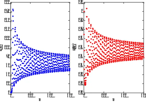
By using the conditions of Theorem 1, we can also see thatD > 0. This completes the proof. Now we can use parameters value in Table 1 for the testing the conditions of Theorem 1. Using these parameter values, it is observed that the positive equilibrium

point(x, y) = (7.41019,0.5599) is local asymptotically stable where blue and red graphs represent x(n) and y(n) population densities respectively (see Figure 1).

Table 1. Parameters values used for numerical analysis

Parameters Numerical Values Ref

μ tumor growth parameter 0.5549 [8]

γ interaction rate 1 [8]

μ tumor stimulated proliferation rate 0.00484 [8]

β inverse threshold for tumor suppression 0.00264 [8]

δ death rate 0.37451 [8]

κ rate of influx 0.19

Figure 1. Graph of the iteration solution ofx(n) and y(n), where x(1) = y(1) = 1

Theorem 2. Let {x(n), y(n)}∞ be a positive solution of the system. Suppose that

μ − γy(n) < 0, βx(n) − 1 > 0 and βμ x(n) y(n) + δy(n) − μ x(n)y(n) − κ < 0 for n =

0,1,2,3 …. Then every solution of (7) is bounded, that is,

x(n) ∈ (0, x(0)) and y(n) ∈ 0,κ

δ .

Proof. Since{x(n), y(n)}∞ > 0 and μ − γy(n) < 0, we have

x(n + 1) = x(n)eμ γ ( ) _{< x(n).}

In addition, if we use βμx(n) y(n) + δy(n) − μ x(n)y(n) − κ < 0 and βx(n) − 1 > 0, we have

y(n + 1) =e μ ( ) βμ ( ) δ _{y(n)(βμ x(n) + δ − μ x(n)) − κ + κ} μx(n)(βx(n) − 1) + δ 0 50 100 150 200 250 300 350 400 450 500 0 1 2 3 4 5 6 7 n x( n) a nd y (n )

<_{μx(n)(βx(n) − 1) + δ <}κ κ_δ.

This completes the proof.

Theorem 3. Let the conditions of Theorem 1 hold and assume that

x <_{2β and y <}1 _{2μ x(n)(βx(n) − 1) + 2δ.}κ If x(n) >1 β and y(n) > κ μx(n)(βx(n) − 1) + δ,

then the positive equilibrium point of the system is global asymptotically stable.

Proof. LetE = (x , y) is a positive equilibrium point of system (7) and we consider a Lyapunov functionV(n) defined by

V(n) = [E(n) − E] , n = 0,1,2 …

The change along the solutions of the system is

∆V(n) = V(n + 1) − V(n) = {E(n + 1) − E(n)}{E(n + 1) + E(n) − 2E}.

Let A = μ − γy(n) < 0 which gives us that y(n) >μ

γ = y. If we consider first equation in (7)

with the factx(n) > 2x , we get

∆V (n) = {x(n + 1) − x(n)}{x(n + 1) + x(n) − 2x} = x(n) e − 1 {x(n)e + x(n) − 2x} < 0.

Similarly, Suppose that A = βμ x(n) + δ − μ x(n) > 0 which yields x(n) >

β. Computations

give us that ify(n) > κ andy(n) > 2 , we have

∆V (n) = {y(n + 1) − y(n)}{y(n + 1) + y(n) − 2y}

= 1 − e _A(κ − y(n)A ) y(n)A e + 1 + κ 1 − e_A − 2yA < 0.

Under the conditions

x <_{2β and y <}1 _{2μ x(n)(βx(n) − 1) + 2δ,}κ

we can write

As a result, we obtain∆V(n) = (∆V (n), ∆V (n)) < 0.

3. NEIMARK-SACKER BIFURCATION ANALYSIS

In this section, we discuss the periodic solutions of the system through Neimark-Sacker bifurcation. This bifurcation occurs of a closed invariant curve from a equilibrium point in discrete dynamical systems, when the equilibrium point changes stability via a pair of complex eigenvalues with unit modulus. These complex eigenvalues lead to periodic solution as a result of limit cycle. In order to study Neimark-Sacker bifurcation we use the following theorem that is called Schur-Cohn criterion.

Theorem B. ([20]) A pair of complex conjugate roots of equation (11) lie on the unit circle and the other roots of equation (11) all lie inside the unit circle if and only if

(a) p(1) = 1 + p + p > 0,

(b) p(−1) = 1 − p + p > 0,

(c) D = 1 + p > 0, (d) D = 1 − p = 0.

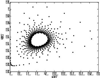
In stability analysis, we have shown that Theorem B/a, Theorem B/b and Theorem B/c always holds. Therefore, to determine bifurcation point we can only analyze Theorem B/d. Solving equation d of Theorem B, we have κ= 0.0635352. Furthermore, Figure 2 shows that κ is the Neimark-Sacker bifurcation point of the system with eigenvalues

λ _, = |0.945907 ± 0.324439i| = 1, where blue, and red graphs represent x(n) and

y(n) population densities respectively.

As seen in Figure 2, a stable limit cycle occurs around the positive equilibrium point at the Neimark-Sacker bifurcation point. This limit cycle leads to periodic solution which means that tumor and immune cell undergo oscillations (Figure 3). This oscillatory behavior has also occurred in continuous biological model as a result of Hopf bifurcation and has observed clinically.

Figure 2. Graph of Neimark-Sacker bifurcation of system (7) for κ= 0.0635352. Initial conditions and 0 20 40 60 80 100 120 140 160 180 200 0.1 0.2 0.3 0.4 0.5 0.6 0.7 0.8 0.9 1 1.1 x(n) y( n)

Figure 3. Graph of the iteration solution of x(n) and y(n) for κ = 0.063535. Initial conditions and other parameters are the same as Figure 1

R

[1] Robert, A.Gatenby, (1995) “Models of tumor-host interaction as competing populations: implications

for tumor biology and treatment”, Journal of Theoretical Biology, Vol. 176, No. 4, pp447-455.

[2] Alberto, D.Onofrio, (2005) “A general framework for modeling tumor-immune system competition

and immunotherapy: mathematical analysis and biomedical inferences”, Physica D-Nonlinear Phenomena, Vol. 208, No. 3-4, pp220-235.

[3] Harold, P.de.Vladar & Jorge, A.Gonzales, (2004) “Dynamic respons of cancer under theinuence of

immunological activity and therapy”, Journal of Theoretical Biology, Vol. 227, No. 3, pp335-348.

[4] Robert, A.Gatenby, (1995) “Models of tumor-host interaction as competing populations: implications

for tumor biology and treatment”, Journal of Theoretical Biology, Vol. 176, No. 4, pp447-455.

[5] Vladimir, A.Kuznetsov, Iliya A.Makalkin, Mark A.Taylor & Alan S.Perelson (1994) “Nonlinear

dynamics of immunogenic tumors: parameter estimation and global bifurcation analysis”, Bulletin of

Mathematical Biology, Vol. 56, No. 2, pp295-321.

[6] N.V, Stepanova, (1980) “Course of the immune reaction during the development of a malignant

tumour”, Biophysics, Vol. 24, No. 5, pp917-923.

[7] Alberto, D.Onofrio, (2008) “Metamodeling tumor-immune system interaction, tumor evasion and

immunotherapy”, Mathematical and Computer Modelling, Vol. 47, No. 5-6, pp614-637.

[8] Alberto, D.Onofrio, Urszula, Ledzewicz & Heinz, Schattler (2012) “On the Dynamics of Tumor

Immune System Interactions and Combined Chemo- and Immunotherapy”, SIMAI Springer Series, Vol. 1, pp249-266.

[9] S. Busenberg, & K.L. Cooke, (1982) “Models of verticallytransmitted diseases with sequential

continuous dynamics”, Nonlinear Phenomena in Mathematical Sciences, Academic Press, New York,

pp.179-187.

[10] Fuat, Gürcan, & Fatma, Bozkurt (2009) “Global stability in a population model with piecewise

constant arguments”, Journal of Mathematical Analysis And Applications, Vol. 360, No. 1,

pp334-342.

[11] Ilhan, Öztürk, Fatma, Bozkurt & Fuat, Gürcan (2012) “Stability analysis of a mathematical modelin a

microcosm with piecewise constant arguments”, Mathematical Bioscience, Vol. 240, No. 2, pp85-91.

0 200 400 600 0 20 40 60 80 100 120 140 160 180 200 n x( n) 0 200 400 600 0.1 0.2 0.3 0.4 0.5 0.6 0.7 0.8 0.9 1 1.1 n y( n)

[12] Ilhan, Öztürk & Fatma, Bozkurt (2011) “Stability analysis of a population model with piecewise

constant arguments”, Nonlinear Analysis-Real World Applications, Vol. 12, No. 3, pp1532-1545.

[13] Fatma, Bozkurt (2013) “Modeling a tumor growth with piecewise constant arguments”, Discrete Dynamics Nature and Society, Vol. 2013, Article ID 841764 (2013).

[14] Kondalsamy, Gopalsamy & Pingzhou, Liu (1998) “Persistence and global stability in a

populationmodel”, Journal of Mathematical Analysis And Applications, Vol. 224, No. 1, pp59-80.

[15] Pingzhou, Liu & Kondalsamy, Gopalsamy (1999) “Global stability and chaos in a population model with piecewise constant arguments”, Applied Mathematics and Computation, Vol. 101, No. 1, pp63-68.

[16] Yoshiaki, Muroya (2008) “New contractivity condition in a population model with piecewise constant

arguments”, Journal of Mathematical Analysis And Applications, Vol. 346, No. 1, pp65-81.

[17] Kazuya, Uesugi, Yoshiaki, Muroya & Emiko, Ishiwata (2004) “On the global attractivity for a logistic

equation with piecewise constant arguments”, Journal of Mathematical Analysis And Applications,

Vol. 294, No. 2, pp560-580.

[18] J.W.H, So & J.S. Yu (1995) “Persistence contractivity and global stability in a logistic equation with

piecewise constant delays”, Journal of Mathematical Analysis And Applications, Vol. 270, No. 2,

pp602-635.

[19] Yoshiaki, Muroya (2002) “Global stability in a logisticequation with piecewise constant arguments”, Hokkaido Mathematical Journal, Vol. 24, No. 2, pp91-108.

[20] Xiaoliang, Li, Chenqi, Mou, Wei, Niu & Dongming, Wang (2011) “Stability analysis for discrete biological models using algebraic methods”, Mathematics in Computer Science, Vol. 5, No. 3, pp247-262.

Authors

Senol Kartal is research assistant in Nevsehir Haci Bektas Veli University in Turkey. He is a Phd student Department of Mathematics, University of Erciyes. His research interests include issues related to dynamical systems in biology.

Fuat Gurcan received her PhD in Accounting at the University of Leeds, UK. He is a Lecturer at the Department of Mathematics, University of Erciyes and International University of Sarajevo. Her research interests are related to Bifurcation Theory, Fluid Dynamics, Mathematical Biology, Computational Fluid Dynamics, Difference Equations and Their Bifurcations. He has published research papers at national and international journals.