https://doi.org/10.1007/s10334-020-00858-0
RESEARCH ARTICLE
Accelerating the co‑simulation method for the design of transmit
array coils for MRI
Alireza Sadeghi‑Tarakameh1,2 · Ehsan Kazemivalipour1,2 · Umut Gundogdu2 · Serhat Erdogan1 · Ergin Atalar1,2
Received: 25 January 2020 / Revised: 18 May 2020 / Accepted: 18 June 2020 / Published online: 27 June 2020 © European Society for Magnetic Resonance in Medicine and Biology (ESMRMB) 2020
Abstract
Objective Accelerating the co-simulation method for the design of transmit array (TxArray) coils is studied using equivalent circuit models.
Materials and methods Although the co-simulation method dramatically reduces the complexity of the design of TxArray coils, finding the optimum solution is not trivial since there exist many local minima in the optimization problem. We propose to utilize an equivalent circuit model of the TxArray coil to obtain a proper initial guess for the optimization process of the co-simulation method. To prove the concept, six different TxArray coils (i.e., three degenerate birdcage coils (DBC), two dual-row head coils, and one elliptical body TxArray coil) with two different loading strategies (cylindrical phantom and human head/body model) at 3 T field strength are investigated theoretically; as an example study, an eight-channel head-DBC is constructed using the obtained values.
Results This approach accelerates the design process more than 20-fold for the coils that are investigated in this manuscript. Conclusion A fast and accurate method for tuning and decoupling of a TxArray coil can be achieved using its equivalent circuit model combined with the co-simulation method.
Keywords MRI · Transmit array · Co-simulation · Inductor calculations · Equivalent circuit model
Introduction
In this work, we introduce a fast method to find the optimum capacitor values for a transmit array (TxArray) coil.
There exist many benefits of using radiofrequency (RF) transmit array coils in magnetic resonance imaging (MRI). One common usage of this technology is for RF-shim-ming [1–4]. For the static magnetic field strength of 3 T or higher, the size of the human body becomes comparable to the wavelength at the Larmor frequency, and homogenous excitation cannot be achieved with the conventional birdcage
body coil. Moreover, the B1+ field is a function of patient
position and size. An array of transmitters can be used to overcome these difficulties. Furthermore, in many RF-shimming applications, the specific absorption rate (SAR) becomes a limiting constraint that can be taken under con-trol by using TxArray coils [5–13]. Another possible use of the TxArray systems is to reduce the duration of the RF pulses designed for complex excitation patterns [14, 15]. As an example, the spatially selective excitation is used for limiting the size of the signal-contributing volume based on the region-of-interest (ROI), which is advantageous for fast data acquisition [16, 17]. Another potential use for the TxArray systems is to achieve implant-friendly MRI scan-ning [18–22].
TxArray coils are studied in many forms, including decoupled strip-lines [23, 24], decoupled surface coils [25,
26], dipole-like structures [27–33] and degenerate birdcage coils (DBC) [34–37]. Despite the advantages of using TxAr-ray coils for MRI, the design and manufacturing of such coils is a significant challenge due to the mutual coupling between elements of the array. One of the practical tech-niques described in the literature is constructing and tuning
Electronic supplementary material The online version of this article (https ://doi.org/10.1007/s1033 4-020-00858 -0) contains supplementary material, which is available to authorized users. * Ergin Atalar
1 Department of Electrical and Electronics Engineering,
Bilkent University, 06800 Ankara, Turkey
2 National Magnetic Resonance Research Center (UMRAM),
only one of the elements, initially, then assembling the remaining elements of the array in successive steps, followed by iteratively tuning and decoupling all elements at each step [34]. Unfortunately, this technique is very time-consuming, making it infeasible for a large number of elements.
The co-simulation method, which was proposed by Kozlov et al. [38], significantly reduced the difficulties of RF coil design methods. In this method, an electromagnetic (EM) simulation is performed by replacing all discrete elements (capacitors and inductors) with excitation ports. The calculated scattering matrix (S matrix) is exported to a circuit simulator in order to optimize the values of these elements. Using this method, the values necessary for tun-ing and decoupltun-ing can be accurately obtained. Addition-ally, it makes large problems (of many independent discrete elements) feasible to solve. However, in the optimization process of this method, the initial guess plays a significant role. In the literature [39, 40], many randomly chosen ini-tial guesses were established to avoid converging to a local minimum, which makes the optimization process time-consuming. On the other hand, there is no guarantee that the optimization will converge to the global minimum using the randomly chosen initial guesses. A pre-calculated initial guess was considered in an earlier study [9], but this strategy was not fully analyzed and did not yield the optimum solu-tion in all cases that were tested.
In this work, we use analytic calculations and finite ele-ment method (FEM)-based simulations to obtain all induc-tive and resisinduc-tive parameters necessary for the organization of the equivalent circuit model. Then, the circuit model is utilized in determining approximate values for the capacitors used in the design. These approximate values of capacitors are used as the initial values for the optimization process of the co-simulation method. To prove the effectiveness of the method, six different TxArray coils with two different load-ing schemes were investigated. The results of the proposed method are compared in terms of accuracy and speed to the results of the conventional co-simulation method with many randomly chosen initial guesses.
Materials and methods
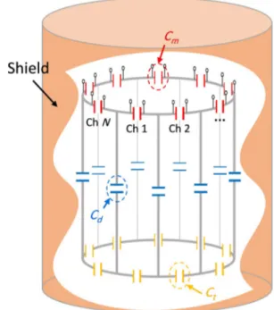
Here, the proposed method will be explained in detail for an N-channel shielded DBC shown in Fig. 1, while, the method can be easily extended for the other types of coils as well. In this design, there are three independent capacitor values: Ct
is the tuning capacitor, Cd is the decoupling capacitor, and Cm is the matching capacitor when the load is a cylindrical uniform phantom.
In the N-channel DBC coil, there are N capacitors of each of the three types. Some capacitors, such as Ct, can be
dis-tributed. The following theory aims to find an approximate
value for each of these capacitors and use them as initial guesses in the optimization process of the co-simulation technique. In the other designs or when the load is not cir-cularly symmetric as in the human head/body model, the numbers of independent capacitor values can be significantly higher.
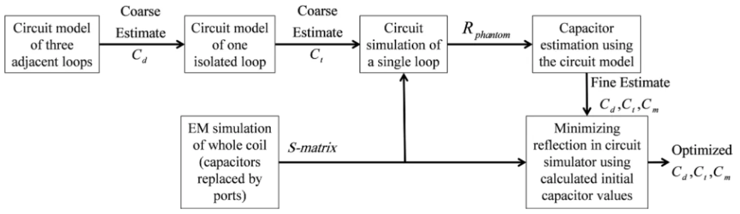
The flowchart of the proposed method is shown in Fig. 2. In this method, we obtain a coarse estimate for the pling and tuning capacitor values, based on the ideal decou-pling between adjacent channels and assuming no loss in the system. Later, these values are used as the initial guesses for the optimization of a simplified circuit model of the array coil. The results of this intermediate optimization process are called the fine estimates. We used these as the initial guesses for the co-simulation method (see Fig. 2). These steps will be described below in detail.
Equivalent circuit model
First, we start with the equivalent circuit model of the coil. By modeling each wire or strip as an inductor—an assumption that is only valid if the wavelength is much larger than the strip segments—a shielded DBC can be modeled as an equivalent circuit that consists of self- and mutual-inductances. Assuming an infinitely long shield, the shield acts as an electromagnetic mirror. Therefore, the shielded DBC can be analyzed using the mirror currents. Finding the position of these mirror currents in a cylindrical coordinate system is a well-known procedure
Fig. 1 An N-channel shielded degenerate birdcage coil. Tunning (Ct),
decoupling (Cd), and matching (Cm) capacitors are shown as three
[41]. We designated the current segments on the coil 1 to 3, and the mirror currents 4 to 6, as shown in Fig. 3a. Let Lj,p,k,q
represent the self- or mutual-inductance of the pth segment in the j th loop with the q th segment in the k th loop. Calculation of each of the inductance values can be found in the existing literature [42, 43]. Kirchhoff’s voltage law for the jth loop can be written in the form of a matrix equation as follows [44]:
where I is a vector of mesh currents, as shown in Fig. 3b. This vector does not include the mirror currents since, by their definition, their values are identical to those of flow on (1) K ⋅ I = 1
𝜔2H ⋅ I
the coil conductors. Therefore, the elements of matrices K and H can be written as [44]:
where 𝛿j,k is the Kronecker delta defined as:
(2) Kj,k= 2(Lj,1,k,1−Lj,1,k,3−Lj,1,k,4+Lj,1,k,6) + 1 ∑ m=0 1 ∑ n=0 (−1)m+n[Lj+m,2,k+n,2−Lj+m,2,k+n,5] (3) Hj,k=2( 1 Ct + 1 Cd ) 𝛿j ,k− (𝛿 j,k+1 Cd + 𝛿j ,k−1 Cd )
Fig. 2 The workflow of the proposed method
Fig. 3 a All combinations of self- and mutual-inductances in the DBC including the image of the coil corresponding to the shield. b The circuit model of three adjacent loops in a DBC was investigated for decoupling and tuning purposes. c Circuit model of a single loop, which was used to determine the loading effect on the coil. d The final equivalent circuit model of the DBC including the loading effect of the phantom
Circuit model of three adjacent loops
In the design of a DBC, decoupling between the channels, tuning to the desired frequency, and impedance matching of the input ports can be considered the essential parameters.
To find the decoupling capacitor value, we ignored the power loss of the phantom and assumed that the coupling between nonadjacent loops (channels) is negligible. Conse-quently, the coupling between adjacent loops with a common rung was canceled using an appropriate capacitor on the common rung. Figure 3b shows the equivalent circuit model of three adjacent loops, such that the loop in the middle (jth loop) is supposed to be decoupled from the (j−1)th and (j + 1)th loops. Therefore, one can obtain a coarse estimate for the decoupling capacitance as shown below.
Circuit model of one isolated loop
To find the tuning capacitor values, we assume perfect decoupling between all channels, no loss (as before), and that the ports are disconnected. Under these assumptions, the array structure can be treated as N separated single loop coils. The Kirchhoff’s voltage law equation for this single loop can simply be written as:
Substituting the value of Cd from Eqs. (5) into (6) and
solving the equation for Ct provides a coarse estimate for the tuning capacitance as follows:
Electromagnetic (EM) simulations of the coil
Similar to the original co-simulation method [38], all of the lumped elements on the coil that are used for tuning, decou-pling, and matching purposes were replaced by 50 Ω ports in an EM simulation environment. The iterative meshing process of the EM simulation was stopped if the greatest (4) 𝛿 j,k= { 1 j = k 0 j ≠ k (5) Cd= − 1 𝜔2K j,j−1 (6) j𝜔 [ Kj,j− 2 𝜔2 ( 1 Ct + 1 Cd )] Ij=0 (7) Ct= 2 𝜔2 ( 1 Kj,j+Kj,j−1+Kj+1,j )
difference between the S-parameters of two successive itera-tions was less than a pre-determined value. Otherwise, the simulator proceeded with finer meshes [45]. Eventually, the S matrix extracted from the EM simulator was imported to a circuit simulator for performing a single-loop circuit simula-tion as well as determining an optimum set of capacitors.
Circuit simulation of a single loop
To obtain a finer estimate of the tuning and decoupling capacitance values and determine an estimate for the match-ing capacitance, the loss (loadmatch-ing effect) is introduced. To predict the loss, a circuit simulation of a single loop was per-formed by assigning zero-capacitance (i.e., large impedance) to lumped elements of all the loops excluding the intended loop. The values obtained for Cd and Ct in Eqs. (5) and (7),
respectively, were used in the single-loop simulation. Based on the circuit model in Fig. 3c, Rphantom was formulated as
follows:
where Zsimulation is the impedance at the port and is
deter-mined by the EM simulator.
Circuit model of all N loops
Once Rphantom is determined, the general equivalent circuit
model for the DBC, including the matching capacitor and loading effect of the phantom (Fig. 3d), can be utilized for design purposes. The impedance matrix corresponding to the circuit model in Fig. 3d can be formulated as follows:
where I is the identity matrix. Then, the scattering matrix of an N-port network, with corresponding impedance matrix Z , can be determined as follows [46]:
where the matrix Z0 represents the characteristic impedance
of transmission lines (50 Ω).
Once the S parameters are calculated, the cost function can be evaluated as the total reflected power from the ports while one of the ports is stimulated by unit power:
(8) Rphantom=real { j 𝜔Cm(j𝜔CmZsimulation−1 ) } (9) Z = − j 𝜔C m [ I + ( j𝜔K − j 𝜔H + RphantomI )−1( j 𝜔C m I )] (10) S = ( Z + Z0I )−1 ⋅ ( Z − Z0I )
We used the steepest-descent method [47, 48] to mini-mize the cost function. If the cost difference between two consecutive iterations is less than a predetermined value, the algorithm is terminated. The final capacitor values become the initial values for the co-simulation method.
After performing the EM simulation, the resultant S matrix was exported to the circuit simulator. In the circuit simulator, each port was connected to its corresponding capacitor. A fine estimate for the capacitors was calculated using the equivalent circuit model introduced above. Uti-lizing the optimization tool of the circuit simulator (which uses the gradient optimization algorithm) with the minimum reflected power constraints and finely estimated capacitor values as the initial guesses, the proper capacitor values were obtained.
Simulations and experiments
To verify the proposed method, six different TxArray coils with two different loading schemes are designed (see Fig. 4) and simulated. One of these designs is constructed and tested with an MRI experiment.
Comparison of the proposed method with the original co‑simulation method
An eight-channel head DBC (Coil 1 in Fig. 4), a 12-channel head DBC (Coil 2 in Fig. 4), a 16-channel cylindrical body DBC (Coil 3 in Fig. 4), a 16-channel dual-row head coil (Coil 4 in Fig. 4), a 16-channel shifted dual-row head coil (Coil 5 in Fig. 4), and a 16-channel elliptical body coil (Coil 6 in Fig. 4) were investigated for proof of the concept. Each (11) Cost = N ∑ n=1 | | Sn1| |
2 structure was investigated in the presence of two different
loading schemes, cylindrical phantom (first row in Fig. 4) and human head/body model (second row in Fig. 4), at 3 T field strength. HFSS (ANSYS, Canonsburg, PA, USA) and Microwave Office (AWR Corp., El Segundo, CA, USA) were used as EM and circuit simulators, respectively. All compu-tations and simulations were performed on a workstation with two quad-core Intel(R) Xeon(R) X5472 processors with a 3 GHz clock rate and 32 GB RAM.
Coil construction
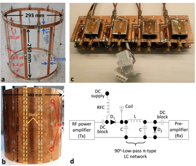
The eight-channel DBC was constructed on a plexiglass cylinder (Fig. 5a) with a diameter of 293 mm. The length of rungs was 250 mm, and the width of copper strips was 15 mm. The RF-shield of the coil was built on a larger plexiglass cylinder (380 mm diameter and 500 mm length) (Fig. 5b). Gradient-induced eddy currents were reduced by slitting the shield in 16 equally spaced locations along the z-direction and connecting them with 1 nF capacitors [49,
50] at the positions facing the end-rings of the coil. We used eight coaxial cables with adjusted bazooka baluns on each cable to carry the RF power from amplifiers to the coil.
The constructed DBC was also used as a receiver by placing a transmit/receive (T/R) switch between the coil, transmit amplifiers, and receiver system. The T/R switch structure and circuit schematic are pictured in Fig. 5c, d, respectively. There are two series-connected PIN diodes; two DC blocking capacitors; an RF choke (RFC), and a 90° low-pass π-type LC network [51]. The scanner provides DC control signals to change the states of the switch. The DC signals are connected to the board by the RFCs. In the transmit mode, the scanner turns on the PIN diodes with a 100 mA current. The receive port is isolated utilizing the high impedance created by the shorted 90° π-network,
Fig. 4 Comparison between the modified and original co-simulation method. Coil 1: eight-channel head DBC, Coil 2: 12-channel head DBC, Coil 3: 16-channel body DBC, Coil 4: 16-channel dual-row head coil, Coil 5: 16-channel shifted dual-row head coil, and Coil 6: 16-channel elliptical body coil. All structured were investigated in the presence of a cylindrical phantom (first row) as well as head/body model (second row)
which acts like a shorted quarter-wave transmission line. In the receive mode, the PIN diodes are turned off with a − 30 V signal so that the receiver port is connected to the coil over the low-pass LC network. The transmitting port is isolated using the high impedance created by the PIN diode, which is in the on-state. The isolation values are approximately 27 dB for both switching states, as deter-mined by means of a bench-top measurement using a net-work analyzer (Agilent-E5061B, Baltimore, MD, United States).
System configurations
The parallel excitation was performed on a 3 T Tim Trio system (Siemens Medical Solutions, Erlangen, Germany) equipped with an 8-channel transmit array system. Each channel used a separate 8 kW RF amplifier (Analogic Corp., Boston, MA, USA). All of the experiments were performed
using a 150 mm diameter cylindrical SNR phantom (3.37 g/L NiCl2.6H2O and 2.4 g/L NaCl), which possessed electrical properties of εr = 80 and σ = 0.62 S/m to mimic the
human head. The conductivity of the phantom was measured using a magnetic resonance electrical properties tomography (MREPT) [52, 53] experiment, and its relative permittivity was assumed to be the same as water.
B1 field mapping and sequence parameters
B1+-maps were acquired using the Bloch-Siegert (BS)
approach described by Sacolick et al. [54] A gradient-echo (GRE) pulse sequence was modified to apply Bloch-Siegert (BS) shift to spins by an off-resonance Fermi pulse. The duration and the off-resonance frequencies were selected to be 8 ms and 2 kHz, respectively. The other relevant imag-ing parameters were TR = 100 ms, TE = 12 ms, NEX = 1, 128 × 128, FOV = 200 mm. Each map was acquired individu-ally in transmit mode, i.e., both slice selection and BS pulses
Fig. 5 Experimental setups. a An eight-channel DBC, which was designed and constructed using the proposed method. b An RF-shield with several parallel slots in the z-direction on it (for reducing
the eddy current effects); c The custom T/R switch used in the MRI experiment, d and the circuit model of the T/R switch
were applied to each channel in transmission mode, one by one. To prevent unreliable data (low-SNR) from affecting the B1-maps, a mask with a threshold of one-tenth of the
maximum B1 value was implemented on the maps. After-ward, a quadrature interpolation was applied to the maps to smoothen them. All of the channels were used for reception, and a sum-of-squares method was used for image recon-struction. Acquired data were analyzed with the method described by Turk et al. [55]. The B1+ relative phase maps
were acquired by simply applying a GRE sequence with the same parameters, except for the Fermi pulse. The reference phase image was taken with the same GRE sequence when all channels were transmitting. The B0 maps were acquired
by a built-in field map sequence using the same imaging parameters, except with a TE1 of 5 ms and TE2 of 12.46 ms.
Results
The performance improvement in the proposed modification to the co-simulation technique is demonstrated by compar-ing the original method to the modified technique.
Comparison of the proposed method with the original co‑simulation method
As a reminder, in the original co-simulation technique, the capacitor values are found using an optimization technique, and the cost function (the total reflected power when unit input is provided from one of the channels of the DBC) is
a nonlinear function of the capacitor values and has many local minima. Because of this difficulty, the optimization problem is solved by repeatedly using the steepest-descent method with different initial guesses and reporting the mini-mum of each solution as the global minimini-mum, as described in the literature [39, 40].
In our proposed method, to find the capacitor values of the DBC, the equivalent circuit model was used as described in the previous section. In the case of the eight-channel head DBC shown in Fig. 5a, analytic calcula-tions led to coarse estimates of 12.9 pF and 24.5 pF for Cd
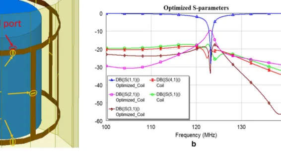
and Ct, respectively. Then, an EM simulation of a single loop in the presence of the phantom was performed, and Rphantom was determined to be 3.8 Ω. Afterward, an inter-stage optimization was performed to obtain a fine estimate for the three capacitor values. At this stage, Cd, Ct, and Cm were computed and found to be 13.9 pF, 8.8 pF, and 89.5 pF, respectively. In the next step, all of the capaci-tors on the coil were replaced by 50 Ω lumped ports in the simulation environment (Fig. 6a). The EM simulation was performed using the iterative meshing technique with 2.5 × 10⁻³ stop criterion (i.e., the difference between the
S-parameters of two successive iterations) which led to 184,000 tetrahedral meshes in the last meshing step. After performing the EM simulation, the resultant S matrix was exported to the circuit simulator. In the circuit simulator, each port was connected to the corresponding capacitor. Utilizing the optimization tool of the circuit simulator, which uses the gradient optimization algorithm, with the minimum reflected power constraints, the proper capacitor
Fig. 6 The procedure of the modified co-simulation method. a The EM simulation model of the DBC, including the phantom, used to extract the S-parameters when all capacitors were replaced with 50 Ω
ports. b The optimized S-parameters using the circuit simulator with the constraint of minimum reflected power
values were obtained. The fine estimates for the capacitor values from the previous stage were used as the initial guesses for the optimization tool at the current stage. The optimized capacitor values were 14.9 pF, 8.4 pF, and 90 pF for Cd, Ct, and Cm, respectively. Figure 6b shows the S-parameters obtained from the circuit simulator.
To compare the efficiency of the proposed method to the original co-simulation method, we repeated the original co-simulation design process as described in the literature [38–40].
All random values were chosen using the rand command in MATLAB (The MathWorks, Natick, MA, USA). By ran-domly choosing 1000 initial guesses (triple-sets of capacitor values in the range of 1 pF to 100 pF), the optimization tool converged to various final cost values. Figure 7a shows the converged cost values for different initial guesses. All circle markers correspond to the randomly chosen initial guesses, and the asterisk marker represents the cost value that was determined by considering the fine estimate for the initial capacitor values. This shows that finding the global mini-mum using randomly chosen initial guesses is not guaran-teed, and it was achieved only three times by seeding with 1000 initial points. On the other hand, the global minimum was found in a single shot when the calculated initial values for the capacitors were used. The total reflected power from all ports for a given global minimum cost value was found by both methods to be 0.25.
The duration of the optimization becomes an important factor for large problems. Figure 7b demonstrates the num-ber of iterations required for different initial guesses. The total number of iterations for 1000 randomly chosen initial guesses was over 794,000. However, the use of the calcu-lated initial value provides the same results in 123 iterations. Thus, in this case study, the proposed algorithm speeds up the optimization process by more than 6400 times.
In Fig. 7c, the final cost values for various initial guesses were plotted with respect to the number of iterations. The cross marker, corresponding to the calculated initial values, provides the minimum cost value achieved using the fewest iterations.
To prove the concept, six different structures, shown in Fig. 4, with two different loading schemes, were investi-gated. The duration for each stage of the design for both methods is given in Table 1. Modified and original co-simulation methods were abbreviated as “M” and “O” in Table 1, respectively. Coils 1 through 6 refer to the struc-tures shown in Fig. 4. The number of independent capacitors represents the number of independent variables that were optimized to achieve the minimum cost function.
In all cases, the number of initial capacitor values (seeds) was chosen to be 1000 to ensure that the global minimum would be achieved. This number is comparable to that used by Kozlov et al. [39, 40] (3000 seeds). For each of the initial capacitor values (seeds), the gradient optimization tool, with
Fig. 7 Analytically calculated initial value vs. randomly cho-sen initial values. a Final cost values achieved using various initial values in the optimization tool. b The number of iterations needed for the optimization tool to converge using various initial values. c The final cost values with respect to the numbers of iterations for different initial values. d The reliable initial guesses in the vicinity of the desired capacitor values that promised to converge to the global minimum
termination constraints of a maximum of 5000 iterations and a convergence tolerance of 10–4, was utilized.
As we argued, if the initial guess in a complex optimiza-tion problem is close to the global minimum, the problem
can be solved using a simple optimization algorithm. In the case of the eight-channel DBC, to determine how close is close enough, the initial guesses for the three capacitor val-ues are scanned between 4 to 14 pf for Ct, 85 pf to 100 pf
Table 1 Comparison between the design duration of the original co-simulation method and the proposed method Number of
independent capacitors
Analytic
calculations EM simulation of the whole coil Circuit simulation of a single loop
Interstage
optimization Final optimization Total Coil 1 Phantom O 3 – 40 min – – 13.5 h ≈ 14 h M 3 < 1 s 40 min < 1 s 15 s 15 s ≈ 40 min Head O 17 – 35 min – – 46 h ≈ 47 h M 17 < 1 s 35 min 4 s 90 s 200 s ≈ 40 min Coil 2 Phantom O 3 – 80 min – – 18.5 h ≈ 20 h M 3 < 1 s 80 min < 1 s 20 s 25 s ≈ 1.5 h Head O 25 – 115 min – – 53 h ≈ 55 h M 25 < 1 s 115 min 5 s 3 min 300 s ≈ 2 h Coil 3 Phantom O 3 – 140 min – – 22.5 h ≈ 25 h M 3 < 1 s 140 min < 1 s 30 s 30 s ≈ 2.5 h Body O 33 – 220 min – – 71 h ≈ 74.5 h M 33 < 1 s 220 min 5 s 5 min 400 s ≈ 4 h Coil 4 Phantom O 4 – 140 min – – 26 h ≈ 28.5 h M 4 < 1 s 140 min < 1 s 40 s 40 s ≈ 3 h Head O 34 – 195 min – – 93.5 h ≈ 97 h M 34 < 1 s 195 min < 1 s 6 min 425 s ≈ 3.5 h Coil 5 Phantom O 4 – 140 min – – 25 h ≈ 27.5 h M 4 < 1 s 140 min < 1 s 40 s 40 s ≈ 2.5 h Head O 34 – 160 min – – 97.5 h ≈ 100 h M 34 < 1 s 160 min < 1 s 6 min 400 s ≈ 3 h Coil 6 Phantom O 12 – 240 min – – 55 h ≈ 59 h M 12 < 1 s 240 min < 1 s 2 min 100 s ≈ 4 h Body O 36 – 250 min – – 174 h ≈ 178 h M 36 < 1 s 250 min < 1 s 6 min 450 s ≈ 4.5 h
for Cm, and 10 pf to 18 pf for Cd. For this example-case, the
initial capacitor values that fall into the volume shown in Fig. 7d, the minimum value was obtained using the steepest descent algorithm is the global minimum. The red diamond shown in the figure represents the fine estimate of the initial capacitor values that is within this volume.
DBC implementation
The nonideal construction of the coil and tolerances of the capacitor values result in slight changes in the resonance frequency (~ 1 MHz) and matching. The capacitors, placed on the upper ring, were used for matching purposes (Cm) and
the value of each of these capacitors was 90 pF. The variable capacitors on the lower ring were utilized as tuning capaci-tors (Ct) and trimmed between 7.5 and 9.5 pF for fine-tuning.
Finally, for decoupling purposes, 14.9 pF capacitors were used on the rungs of the coil (Cd).
Table 2 shows reflection and coupling coefficients in dB for the DBC at 123.2 MHz. All numbers in Table 2a were obtained by bench-top measurement of the S-parameters of the constructed coil using the network analyzer. The maxi-mum of the reflection coefficient (Snn) was − 28 dB. In the
worst case, the mutual coupling coefficient (Smn) for the
adjacent channels was − 11 dB. However, for nonadjacent channels, it was − 18 dB. Table 2b shows the S-parameters obtained in the EM simulation environment for the corre-sponding DBC.
The ratio of total reflected power to input power was 18% in the case of the constructed DBC but was 25% in the simu-lation environment. The difference between simulated and measured reflection values is possibly due to a mismatch between the geometry of the constructed coil and the simu-lation model. Besides, the capacitors were modeled as loss-less in the EM simulations. The equivalent series resistance of the capacitors that we used may also play a role in this small error.
Table 2 Scattering parameters of the DBC. (a) Experimentally measured. (b) Obtained from the EM simulation Channel 1 2 3 4 5 6 7 8 Experiment 1 − 28 2 − 11 − 29 3 − 29 − 12 − 29 4 − 21 − 29 − 11 − 30 5 − 19 − 20 − 30 − 11 − 28 6 − 20 − 18 − 20 − 29 − 12 − 29 7 − 30 − 21 − 19 − 20 − 30 − 11 − 29 8 − 12 − 29 − 20 − 18 − 20 − 29 − 11 − 28 Simulation 1 − 30 2 − 9.6 − 30 3 − 30 − 9.6 − 26 4 − 21 − 29 − 9.6 − 27 5 − 19 − 21 − 29 − 9.6 − 28 6 − 21 − 19 − 21 − 29 − 9.6 − 25 7 − 30 − 21 − 19 − 21 − 29 − 9.6 − 32 8 − 10 − 30 − 21 − 19 − 21 − 31 − 9.6 − 28
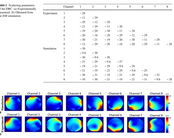
Field maps
Once the B1+ maps are known, the TxArray system can be
utilized for many applications, such as RF shimming [1–4]. The maps were acquired using the technique discussed in the Methods and Materials section. Figure 8 shows both the simulated and measured maps.
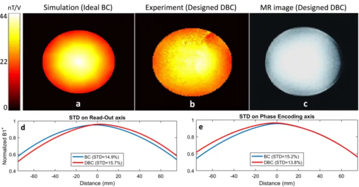
To provide proof of proper operation of the DBC, we implemented RF shimming. To do so, we performed an EM simulation related to an ideal birdcage coil (BC) with the same size as the designed DBC. Quadrature excitation was used in the simulation environment to excite the circularly polarized (CP) mode of the BC (Fig. 9a). In the shimming process, we considered the B1+ profile corresponding to the
CP mode as the desired profile. We optimized the phase and magnitude for each channel using the steepest descent method. In this proof-of-operation study, we did not include the power criterion in the optimization problem. Panels a and b of Fig. 9 demonstrate the simulated and measured B1+-maps for the desired CP mode and the optimized
pro-file, respectively. Figure 9c is a gradient-echo MR image obtained using the optimized excitations.
The comparison between the homogeneity performance of the BC and DBC can be investigated using the stand-ard deviation of the B1+ inside the phantom. Figure 9d
demonstrates the relative standard deviation of B1+ on the
readout axis for both the BC and DBC. Similarly, Fig. 9e shows the same parameter for both coils on the phase encod-ing axis. Accordencod-ingly, the relative standard deviation on the readout axis was 14.9% and 15.7% for the BC and DBC, respectively. On the phase encoding axis, this was 15.2% and 13.8%, respectively, for the BC and DBC. These results indicate that we managed to design DBC as desired, that is it has a mode of operation very similar to BC.
Discussion
In this paper, accelerating the co-simulation method for the design of TxArray coils is studied using equivalent circuit models. In the original co-simulation method proposed by Kozlov et al. [38], an EM simulation of the coil in the pres-ence of an imaging object is performed while all lumped ele-ments are replaced by excitation ports. Afterward, the result-ant S-parameters are imported to a circuit simulator and a time-consuming optimization is performed on the lumped element values, due to the excessive number of local minima in the problem. In the proposed method, we show that start-ing from proper initial guesses for the capacitor values in the optimization process helps in quickly finding the optimum
Fig. 9 a B1+-map of CP-mode of a standard BC that was achieved
using the proper EM simulation. b CP mode that was generated using the constructed DBC. c The GRE image taken from a uniform phantom using the DBC. The sequence parameters are TR = 100 ms, TE = 12 ms, NEX = 1, 128 × 128, FOV = 20 cm, and slice
thick-ness = 5 mm. d, e The standard deviation of B1+ on readout and phase
encoding axes corresponding to both BC and DBC. Calculated mean standard deviations (in percentage) verify a good performance of the DBC
capacitor values. As an example, an eight-channel head-degenerate birdcage coil is constructed using the obtained values, during which the design process is accelerated by a factor of 20.
As shown in Table 1, the acceleration occurs in the final optimization stage of the design process. Correspondingly, the acceleration factor mostly depends on the number of unknown parameters (capacitor values) during the optimi-zation. In the case of the coils in Fig. 4 in the presence of the cylindrical phantom, the number of independent capaci-tors was decreased to three, three, three, four, four, and 12, respectively, due to the cylindrical symmetry. However, in the case of the loading with the human model, these num-bers were 17, 25, 33, 34, 34, and 36, respectively. Note that, to assign the independent optimization parameter to the decoupling capacitors, we only considered the geometrical features of the coils regardless of the loading schemes.
Currently, degenerate birdcage coils are not used exten-sively in ultra-high field applications. However, these coils are one of the best choices for a 3 T transmit array coil because it has a mode of operation similar to a conven-tional birdcage coil. Unfortunately, the complexity of their design is a disadvantage. This manuscript partially addresses this problem, as well. Although we presented the circuit model for DBCs and used the corresponding circuit models for five other types of TxArray coils in this work, the proposed method can be easily extended and utilized in the design of other types of TxArray coils, as well, using a proper equivalent circuit model for the intended coil. The corresponding MATLAB scripts for the presented examples (i.e., six different coils with two different load-ing schemes) which include a relatively large variety of TxArrays to prove the concept are available online as the supplementary material.
It should be noted that in the presented equivalent circuit model, the inductors represent the copper strips of the coil. However, this representation is only valid if the wavelength is much greater than the size of the strips. As the length of the wire increases, a multistage RLC network or even more complex models may be necessary to model a single conduc-tive strip [51].
Furthermore, determining the optimum geometry of the TxArray coils in terms of either their dimensions or their shape is always demanding. Since tuning and decoupling of a candidate geometry is usually a time-consuming process, it is difficult to explore the many varieties of possible geom-etries. The proposed method can shorten the design process and determine the feasibility of a design, allowing a greater number of candidate designs to be examined.
The workstation used in this study is a mediocre system with enhanced memory. Clearly, more powerful systems can make the design process faster. Additionally, the gradi-ent descgradi-ent method we used as an optimization algorithm
may not be the best choice for this problem. There are many sophisticated minimization algorithms for problems involv-ing multiple local minima. As can be understood from Fig. 7, this problem has many local minima. Here, instead of optimizing the optimization algorithm, we chose to work on the minimization of the search interval. Our proposed solution should also help all other optimization algorithms since the initial guess is close to the optimum point.
In the construction of the coil, fine adjustment of the tun-ing capacitors was necessary. We believe this is mainly due to tolerances in the capacitors and imperfections in their construction. These can be handled by measuring the capaci-tance errors and 3D printing the coil-housing. Some addi-tional errors are due to the errors of the EM simulations. To reduce these errors, convergence criteria can be reduced, though this significantly increases the simulation time and the memory requirement. However, the errors due to EM simulation are significantly fewer in number than those due to other sources of error.
Acknowledgements This project was supported by ASELSAN A.S. Ankara, Turkey. MREPT experiments were performed by the aid of Mr. Safa Ozdemir using the facilities of UMRAM, Bilkent University, Ankara, Turkey.
Author contributions AST: responsible for study conception and design, acquisition of data, analysis and interpretation of data, and drafting of manuscript. EK: involved in study conception and design. UG: advised and developed methods for the acquisition of data. SE: advised and developed methods to analyze the data. EA: responsible for study conception and design, analysis and interpretation of data, drafting of the manuscript, and critical revision of the manuscript.
Compliance with ethical standards
Conflict of interest The authors declare that they have received a re-search grant from ASELSAN.
Ethical approval The editorial does not contain any studies with human participants or animals performed by any of the authors.
Human and animal rights This article does not contain any studies with human participants or animals performed by any of the authors.
References
1. Tropp J (2004) Image brightening in samples of high dielectric constant. J Magn Reson 167(1):12–24
2. Bernstein MA, Huston J, Ward HA (2006) Imaging artifacts at 3.0 T. J Magn Reson Imaging 24(4):735–746
3. Childs AS, Malik SJ, O’Regan DP, Hajnal JV (2013) Impact of number of channels on RF shimming at 3T. Magn Reson Mater Biol Phy Med 26(4):401–410
4. Setsompop K, Wald LL, Alagappan V, Gagoski B, Hebrank F, Fontius U, Schmitt F, Adalsteinsson E (2006) Parallel RF transmission with eight channels at 3 Tesla. Magn Reson Med 56(5):1163–1171
5. Guérin B, Gebhardt M, Cauley S, Adalsteinsson E, Wald LL (2014) Local specific absorption rate (SAR), global SAR, trans-mitter power, and excitation accuracy trade-offs in low flip-angle parallel transmit pulse design. Magn Reson Med 71(4):1446–1457 6. Cloos MA, Luong M, Ferrand G, Amadon A, Le Bihan D, Boulant
N (2010) Local SAR reduction in parallel excitation based on channel-dependent Tikhonov parameters. J Magn Reson Imaging 32(5):1209–1216
7. Zhu Y, Alon L, Deniz CM, Brown R, Sodickson DK (2012) Sys-tem and SAR characterization in parallel RF transmission. Magn Reson Med 67(5):1367–1378
8. van den Bergen B, Van den Berg CA, Bartels LW, Lagendijk JJ (2007) 7 T body MRI: B1 shimming with simultaneous SAR reduction. Phys Med Biol 52(17):5429
9. Guérin B, Gebhardt M, Serano P, Adalsteinsson E, Hamm M, Pfeuffer J, Nistler J, Wald LL (2015) Comparison of simulated parallel transmit body arrays at 3 T using excitation uniform-ity, global SAR, local SAR, and power efficiency metrics. Magn Reson Med 73(3):1137–1150
10. Lattanzi R, Sodickson DK, Grant AK, Zhu Y (2009) Elec-trodynamic constraints on homogeneity and radiofrequency power deposition in multiple coil excitations. Magn Reson Med 61(2):315–334
11. Sadeghi-Tarakameh A, Torrado-Carvajal A, Ariyurek C, Atalar E, Adriany G, Metzger G, Lagore R, DelaBarre L, Grant A, Van de Moortele P, Ugurbil K, Eryaman Y (2018) Optimizing the topography of transmit coils for SAR management. In: Proceed-ing of the 26th Joint Annual MeetProceed-ing ISMRM-ESMRMB, Paris, France. p 0297
12. Sadeghi-Tarakameh A, DelaBarre L, Lagore RL, Torrado-Carvajal A, Wu X, Grant A, Adriany G, Metzger GJ, Van de Moortele PF, Ugurbil K, Atalar E, Eryaman Y (2020) In vivo human head MRI at 10.5 T: A radiofrequency safety study and preliminary imaging results. Magn Reson Med 84(1):484–496
13. Sadeghi-Tarakameh A, Wu X, Ulus F, Eryaman Y, Atalar E (2019) Ultimate Intrinsic Specific Absorption Rate Efficiency. In: Pro-ceedings of the 27th Annual Meeting of ISMRM, Montreal, QC, Canada. p 4166
14. Katscher U, Börnert P (2006) Parallel RF transmission in MRI. NMR Biomed 19(3):393–400
15. Zhu Y (2004) Parallel excitation with an array of transmit coils. Magn Reson Med 51(4):775–784
16. Pauly J, Nishimura D, Macovski A (1989) A linear class of large-tip-angle selective excitation pulses. J Magn Reson 82(3):571–587 17. Hardy CJ, Cline HE (1989) Spatial localization in two dimensions
using NMR designer pulses. J Magn Reson 82(3):647–654 18. Eryaman Y, Akin B, Atalar E (2011) Reduction of implant RF
heating through modification of transmit coil electric field. Magn Reson Med 65(5):1305–1313
19. Eryaman Y, Guerin B, Akgun C, Herraiz JL, Martin A, Tor-rado-Carvajal A, Malpica N, Hernandez-Tamames JA, Schiavi E, Adalsteinsson E (2015) Parallel transmit pulse design for patients with deep brain stimulation implants. Magn Reson Med 73(5):1896–1903
20. Eryaman Y, Turk EA, Oto C, Algin O, Atalar E (2013) Reduction of the radiofrequency heating of metallic devices using a dual-drive birdcage coil. Magn Reson Med 69(3):845–852
21. Kazemivalipour E, Keil B, Vali A, Rajan S, Elahi B, Atalar E, Wald LL, Rosenow J, Pilitsis J, Golestanirad L (2019) Recon-figurable MRI technology for low-SAR imaging of deep brain stimulation at 3T: application in bilateral leads, fully-implanted systems, and surgically modified lead trajectories. NeuroImage 199:18–29
22. Golestanirad L, Kazemivalipour E, Keil B, Downs S, Kirsch J, Elahi B, Pilitsis J, Wald LL (2019) Reconfigurable MRI coil technology can substantially reduce RF heating of deep brain
stimulation implants: first in-vitro study of RF heating reduction in bilateral DBS leads at 1.5 T. PLoS ONE 14:8
23. Lee RF, Hardy CJ, Sodickson DK, Bottomley PA (2004) Lumped-element planar strip array (LPSA) for parallel MRI. Magn Reson Med 51(1):172–183
24. Adriany G, de Moortele V, Wiesinger F, Moeller S, Strupp JP, Andersen P, Snyder C, Zhang X, Chen W, Pruessmann KP (2005) Transmit and receive transmission line arrays for 7 Tesla parallel imaging. Magn Reson Med 53(2):434–445
25. Roemer PB, Edelstein WA, Hayes CE, Souza SP, Mueller O (1990) The NMR phased array. Magn Reson Med 16(2):192–225 26. Wu B, Qu P, Wang C, Yuan J, Shen GX (2007) Interconnecting
L/C components for decoupling and its application to low-field open MRI array. Conc Magn Reson Part B Magn Reson Eng 31(2):116–126
27. Raaijmakers AJE, Ipek O, Klomp DWJ, Possanzini C, Harvey PR, Lagendijk JJW, van Den Berg CAT (2011) Design of a radiative surface coil array element at 7 T: the single-side adapted dipole antenna. Magn Reson Med 66(5):1488–1497
28. Raaijmakers AJE, Italiaander M, Voogt IJ, Luijten PR, Hoogduin JM, Klomp DWJ, van Den Berg CAT (2016) The fractionated dipole antenna: a new antenna for body imaging at 7 T esla. Magn Reson Med 75(3):1366–1374
29. Steensma B, Andrade A, Klomp D, Van den Berg C, Luijten P, Raaijmakers (2016) A Body imaging at 7 Tesla with much lower SAR levels: an introduction of the Snake Antenna array. In: Pro-ceedings of the 24th Annual Meeting of ISMRM, Singapore. p 0395
30. Ertürk MA, Wu X, Eryaman Y, Van de Moortele PF, Auerbach EJ, Lagore RL, DelaBarre L, Vaughan JT, Uğurbil K, Adriany G (2017) Toward imaging the body at 10.5 tesla. Magn Reson Med 77(1):434–443
31. Sadeghi-Tarakameh A, Adriany G, Metzger GJ, Lagore RL, Jun-gst S, DelaBarre L, Van de Moortele PF, Ugurbil K, Atalar E, Eryaman Y (2020) Improving radiofrequency power and specific absorption rate management with bumped transmit elements in ultra‐high field MRI. Magn Reson Med. https ://doi.org/10.1002/ mrm.28382
32. Sadeghi-Tarakameh A, Jungst S, Wu X, Lanagan M, Adriany G, Metzger GJ, Van de Moortele P-F, Ugurbil K, Atalar E, Eryaman Y (2019) A New Coil Element for Highly-Dense Transmit Arrays: An Introduction to Non-Uniform Dielectric Substrate (NODES) Antenna. In: Proceedings of the 27th Annual Meeting of ISMRM, Montreal, QC, Canada. p 0732
33. Sadeghi-Tarakameh A, Torrado-Carvajal A, Lagore RL, Moen S, Wu X, Adriany G, Metzger GJ, DelaBarre L, Ugurbil K, Ata-lar E, Eryaman Y (2019) Toward Human Head Imaging at 10.5 T Using an Eight-Channel Transmit/Receive Array of Bumped Fractionated Dipoles. In: Proceedings of the 27th Annual Meeting of ISMRM, Montreal, QC, Canada. p 0430
34. Alagappan V, Nistler J, Adalsteinsson E, Setsompop K, Fontius U, Zelinski A, Vester M, Wiggins GC, Hebrank F, Renz W (2007) Degenerate mode band-pass birdcage coil for accelerated parallel excitation. Magn Reson Med 57(6):1148–1158
35. Stara R, Tiberi G, Morsani F, Symms M, Fantacci ME, Marletta M, Zampa V, Pendse M, Retico A, Rutt BK (2017) A degenerate birdcage with integrated Tx/Rx switches and butler matrix for the human limbs at 7 T. Appl Magn Reson 48(3):307–326
36. Sadeghi-Tarakameh A, Kazemivalipour E, Demir T, Gundogdu U, Atalar E (2018) Accelerating the Co-Simulation Method for Fast Design of Transmit Array Coils: An Example Study on a Degenerate Birdcage Coil. In: Proceeding of the 26th Joint Annual Meeting ISMRM-ESMRMB, Paris, France. p 4404
37. Kazemivalipour E, Sadeghi Tarakameh A, Yilmaz U, Acikel V, Sen B, Atalar E (2018) A 12-channel degenerate birdcage body transmit array coil for 1.5T MRI scanners. In: Proceeding of the
26th Joint Annual Meeting ISMRM-ESMRMB, Paris, France. p 1708
38. Kozlov M, Turner R (2009) Fast MRI coil analysis based on 3-D electromagnetic and RF circuit co-simulation. J Magn Reson 200(1):147–152
39. Kozlov M, Turner R Analysis of RF transmit performance for a multi-row multi-channel MRI loop array at 300 and 400 MHz. In: Microwave Conference Proceedings (APMC), 2011 Asia-Pacific, 2011. IEEE, pp 1190–1193
40. Kozlov M, Turner R Analysis of RF transmit performance for a 7T dual row multichannel MRI loop array. In: Engineering in Medicine and Biology Society, EMBC, 2011 Annual International Conference of the IEEE, 2011. IEEE, pp 547–553
41. Cheng DK (1993) Fundamentals of engineering electromagnetics. Pearson Education, New Jersey, pp 136–142
42. Grover FW (2004) Inductance calculations: working formulas and tables. Dover Publication, New York, pp 20–76
43. Tarakameh AS (2016) Design of a birdcage-like radio frequency transmit array coil for the magnetic resonance imaging using equivalent circuit model. Bilkent University, Thesis
44. Jin J (1998) Electromagnetic analysis and design in magnetic reso-nance imaging, vol 1. CRC Press, Florida
45. Kozlov M, Turner R (2010) A comparison of Ansoft HFSS and CST microwave studio simulation software for multi-channel coil design and SAR estimation at 7T MRI. Piers Online 6(4):395–399 46. Pozar DM (2009) Microwave engineering, 2nd edn. John Wiley
& Sons, New York, pp 182–244
47. Habashy TM, Abubakar A (2004) A general framework for con-straint minimization for the inversion of electromagnetic measure-ments. Progr Electromagn Res 46:265–312
48. Etminan A, Sadeghi A, Gurel L (2014) Electromagnetic imaging of three-dimensional dielectric objects with Newton minimiza-tion. In: Antennas and Propagation Society International Sympo-sium (APS-URSI), IEEE, p 876–877
49. Hayes CE, Eash MG (1987) Shield for decoupling RF and gradient coils in an NMR apparatus. Google Patents
50. Roemer PB, Edelstein WA (1989) RF shield for RF coil contained within gradient coils of NMR imaging device. Google Patents 51. Bahl IJ (2003) Lumped elements for RF and microwave circuits.
Artech house, Boston
52. Hafalir FS, Oran OF, Gurler N, Ider YZ (2014) Convection-reaction equation based magnetic resonance electrical prop-erties tomography (cr-MREPT). IEEE Trans Med Imaging 33(3):777–793
53. Gurler N, Ider YZ (2017) Gradient-based electrical conductivity imaging using MR phase. Magn Reson Med 77(1):137–150 54. Sacolick LI, Wiesinger F, Hancu I, Vogel MW (2010) B1 mapping
by Bloch-Siegert shift. Magn Reson Med 63(5):1315–1322 55. Turk EA, Ider YZ, Ergun AS, Atalar E (2015) Approximate
Fou-rier domain expression for Bloch-Siegert shift. Magn Reson Med 73(1):117–125
Publisher’s Note Springer Nature remains neutral with regard to jurisdictional claims in published maps and institutional affiliations.