Estimating the glossiness transfer function induced
by illumination change and testing its transitivity
Department of Psychology, Bilkent University, Ankara, Turkey, & National Research Center for Magnetic Resonance (UMRAM), Bilkent University, Ankara, Turkey
Katja
Doerschner
Department of Psychology, Bilkent University, Ankara, Turkey, & National Research Center for Magnetic Resonance (UMRAM), Bilkent University, Ankara, Turkey
Huseyin
Boyaci
Department of Psychology, New York University, New York, NY, USA, & Center for Neural Science, New York University, New York, NY, USA
Laurence T.
Maloney
The light reflected from a glossy surface depends on the reflectance properties of that surface as well as the flow of light in the scene, the lightfield. We asked four observers to compare the glossiness of pairs of surfaces under two different real-word lightfields, and used this data to estimate a transfer function that captures how perceived glossiness is remapped in changing from one real-world lightfield to a second. We wished to determine the form of the transfer function and to test whether for any set of three lightfields the transfer function from light field 1 to light field 2 and the transfer function from light field 2 to light field 3 could be used to predict the glossiness transfer function from light field 1 to light field 3. Observers’ estimated glossiness transfer functions for three sets of lightfields were best described by a linear model. The estimated transfer functions exhibited the expected transitivity pattern for three out of four observers. The failure of transitivity for one observer, while significant, was less than 12.5% of the gloss range.
Keywords: perception of surface gloss, transitivity, glossiness transfer function, surface material perception, gloss constancy, complex illumination
Citation:Doerschner, K., Boyaci, H., & Maloney, L. T. (2010). Estimating the glossiness transfer function induced by illumination change and testing its transitivity. Journal of Vision, 10(4):8, 1–9, http://journalofvision.org/10/4/8/, doi:10.1167/10.4.8.
Introduction
The perceived glossiness of a material depends on a number of parameters including the specular reflectance of the surface, specular blur, and the angles of the surface normal to the light sources and the line of sight. Hunter and Harold (1987) specified six distinct types of gloss each depending on a specific modification of those parameters. Early studies investigating the perception of surface gloss focused on the properties of specular highlights (Beck, 1972; Beck & Prazdny, 1981; more recently, Berzhanskaya, Swaminathan, Beck, & Mingolla,
2005). A specular highlight however only constitutes a special case of specular reflection (Figure 1A). Those that one usually encounters in daily life in indoor and outdoor settings are by far more complex. Advances in computer graphics (Debevec,1998) have made it possible to capture real-world high dynamic range illuminations and to employ
these illumination maps in realistic renderings of objects and scenes, including glossy materials (Figure 1B).
Research using rendering techniques simulating complex light sources (light fields, Gershun,1939) has shown that perceived glossiness also depends on the spatial distribu-tion and intensity of light sources in the scene (Fleming, Dror, & Adelson, 2003). Fleming et al. (2003) showed that observers are able to match (though not perfectly) the gloss and surface roughness of CRT-displayed, monocu-larly viewed glossy surfaces rendered under two different real-world light fields drawn from a data base of light probes1 collected by Debevec (1998). However matching performance did not indicate that perception of gloss was independent of choice of light field (gloss constancy). Surfaces appeared less glossy under simple light fields generated by a small number of point sources than under real world light fields as those sampled by Debevec.
In summary, Fleming et al. showed that glossiness constancy is not perfect even among complex, real world
illuminations. While making an important contribution to our understanding of the perception of surface gloss, Fleming et al. did not quantify how changes in illumina-tion affected perceived gloss. In this research we charac-terize how perceived glossiness varies as we move from one particular illumination environment to another by introducing the concept of theglossiness transfer function.
The glossiness transfer function&
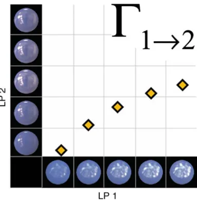
We would like to capture how the perceived glossiness of surfaces changes with changes in illumination. Con-sider Figure 2: A sphere with certain surface reflectance characteristics is rendered at different gloss levels under light probe (LP) 1 and compared to a second sphere with the same reflectance characteristics rendered at the same gloss levels under LP 2. The diamonds on the plot mark the points of perceived equal gloss. For example, the sphere rendered under LP 1 at level 5 is perceived to be as glossy as the sphere under LP 2 at level 3.
These points of equal perceived gloss trace an isogloss contour. We refer to this contour as the glossiness transfer function *1Y2. It describes how perceived glossiness is remapped in changing from one real world light field to a second. That is, if a surface has perceived glossiness g1
under LP 1 then it has perceived glossinessg2=*1Y2(g1)
under LP 2.
In the analysis below we first measure* for 10 different surfaces differing in glossiness under three different real-world light fields.
Second, we test the transitivity of the measured glossiness transfer functions,
*1Y3¼ *2Y3: *1Y2; ð1Þ
where*1Y2 is the glossiness transfer function from LP 1 to LP 2,*2Y3is the glossiness transfer function from LP 2 to LP 3,*1Y3is the glossiness transfer function from LP 1
to LP 3, and ‘:’ denotes composition of functions. That is, for any surface with perceived glossiness g1 under LP 1,
we test whether g3 = *2Y3(*1Y2(g1)) across the range of
surfaces considered.
Intuitively, the transitivity test is a test of an implicit model of how human observers perceive glossiness. Given any surface under any illumination conditions, we assume that the visual system effectively estimates a single scale value that represents the perceived gloss of the surface. These numbers control judgments of glossiness and, in particular, when observers are asked to report which of two stimuli viewed under two light fields is glossier, they pick the stimulus with the higher scale value. If this model is correct, then observers’ judgments will be transitive. A failure of transitivity would lead to rejection of the model just described.
How could the model fail? An evident possibility is that perceived gloss is not univariate but rather multivariate. If for example there are multiple cues to gloss, one based on the sharpness of edges, another on skewness of the intensity histogram (Motoyoshi, Nishida, Sharan, & Adelson, 2007), then the observer, may rely primarily on one glossiness cue in comparing surfaces under LP 1 and LP 2 and switch to a second cue in comparing surfaces under LP 2 and LP 3. If, for example, two light fields are produced by multiple light sources with sharp edges, it would be natural to rely on the sharpness of edges in comparing the glossiness of surfaces. For two light fields that are primarily diffuse, the skewness cue may be selected. If glossiness cues are not highly correlated
Figure 1. The same virtual object rendered under two different illuminants. The sphere is rendered using the model of Ward (1992). A. A collimated source. B. A real-world illuminant measured by Debevec (1998).
Figure 2. An illustration of the glossiness transfer function * for two light probes. Yellow diamonds represent points of perceived equal glossiness.
across surfaces and lighting conditions and the observer switches among cues in this way, there is no reason to expect transitivity. If the observer uses only a single cue or a fixed rule of combination on multiple cues, we expect transitivity.
Fundamentally, the transitivity test is a test of whether we should describe glossiness as a univariate perceptual attribute like lightness (Gilchrist, 2006; Gilchrist & Kossyfidis, 1999) or the result of a dynamic integration of possibly conflicting cues such as perception of depth (Landy, Maloney, Johnston, & Young,1995).
Experiment
Methods
Stimuli
The stimuli were three-dimensional spheres computer-rendered with the Radiance software package (Larson & Shakespeare, 1996). We choose to work with stereo images in order to increase the realism of the renderings. The spheres were rendered under three different high dynamic range real world-illumination maps (Debevec,
1998) at 10 different specularity levels (Figure 3). To achieve different levels of gloss we varied the specular reflectance parameter>s(Ward,1992) from 0.02 to 0.139,
while holding the diffuse component (>d) and surface
roughness (!) constant. The chosen values of >s do not
correspond to perceptually equally spaced values of gloss. Furthermore we did not perform any compression of the luminance values, nor introduced artificial glare to our renderings. If a luminance value was greater than 1, as it is often encountered with high dynamic range illumination maps it was cut off.
Apparatus
The experimental apparatus was a computer-controlled stereoscope. The left and right images were presented to the corresponding eye of the observer on two 21VV Sony Trinitron Multiscan GDM-F500 monitors placed to the observer’s left and right. The screens on these monitors are close to physically flat, with less than 1 mm of deviation across the surface of each
monitor. Two small mirrors were placed directly in front of the observer’s eyes. These mirrors reflected the images displayed on the left and right monitors upon the corresponding eye of the observer (Figure 4).
Look-up tables were used to correct nonlinearities in the gun responses and to equalize the display values on the two monitors. The tables were prepared after direct mea-surements of the luminance values on each monitor with a Photo Research PR-650 spectrometer. The maximum luminance achievable on either screen was 114 cd/m2. The stereoscope was contained in a box 124 cm on a side. The front face of the box was open and that is where the observer sat in a chin/head rest. The interior of the box was coated with black flocked paper (Edmund Scientific) to absorb stray light. Only the stimuli on the screens of the monitors were visible to the observer. The casings of the monitors and any other features of the room were hidden behind the non-reflective walls of the enclosing box.
Additional light baffles were placed near the observer’s face to prevent light from the screens reaching the
Figure 3. A sphere rendered at the 10 gloss levels. The different gloss levels are achieved by varying the specular reflectance parameter >sin the Ward model (Ward,1992).
Figure 4. Computer-controlled stereoscope. The left and right images of each stereo pair were displayed on two monitors placed to the left and the right of the observer. The observer viewed these images reflected in small mirrors directly in front of his or her eyes. The fused image appeared approximately 70 cm in front of the observer, the optical distance to either screen.
observer’s eyes directly. The optical distance from each of the observer’s eyes to the corresponding computer screen was 70 cm. To minimize any conflict between binocular disparity and accommodation depth cues, the spheres were rendered to be exactly 70 cm in front of the observer.
A note on psychophysical method
In a first attempt to find the glossiness transfer function * we used the method of adjustment, that is, we asked the observers for any given pair of spheres to adjust the gloss levels of the left sphere such that it matches the gloss level of the right one. Observers performed this task for all possible LP combinations at every gloss (specularity) levels. For each observer we obtained three pairs of data sets, where in each pair test and match LP were exchanged. For example in one set LP 1 would be used in rendering the test sphere and LP 2 in rendering the match, and, conversely, in a second set LP 1 would be used in rendering the match sphere and LP 2, the test. We would expect that the settings for each pair of surfaces should not depend on whether the test is viewed under LP 1 and the match under LP 2 or vice versa. However, results from 6 observers show strong biases in the results for perceived equal glossiness. A surface is perceived as less glossy when it is the test surface than when it is the matching surface. This asymmetry may be due to a response bias (conservatism), or possibly due to adapta-tion to the gloss level of the test surface. In Figure 5 we show the results for two representative observers. Note, how the measured * deviates from the predicted one. Fleming et al. (2003) used method of adjustment for all of their data and noted this same problem.
We abandoned the adjustment paradigm and replaced it with a two alternative forced choice (2AFC) task in order to avoid the observed response bias and to make
mean-ingful estimates of the effect of different light fields on perceived surface gloss.
Software
The experimental software was written by us in the C language. We used the X Window System, Version 11R6 (Scheifler & Gettys, 1996) running under Red Hat Linux 6.1 for graphical display. The computer was a Dell 410 Workstation with a Matrox G450 dual head graphics card and a special purpose graphics driver from Xi Graphics that permitted a single computer to control both monitors. We use the open source physics-based rendering package Radiance (Larson & Shakespeare,1996) to render the left and right images of the stereo pair for a given virtual scene. The output of the rendering described above was a stereo image pair with floating point RGB triplets for each pixel. These triplets were translated to a 24-bit graphics code, correcting for nonlinearities in the monitors’ responses by means of measured look-up tables for each monitor.
Task
On a given trial the observer was presented with stereo images of a pair of spheres placed side by side, each under a different light field and at a randomly chosen specularity level (Figure 6). The observer was asked to indicate which of the two displayed spheres appeared glossier by pressing the corresponding mouse button. After the button response the next stimulus pair was displayed.
We chose light probes taken from three real-world light fields from the Debevec collection. They had code names Galileo, RNL (taken in a eucalyptus grove at the University of California at Berkley), and St. Peter’s. The first and third light probes were recorded indoors and the
Figure 5. Data for two representative observers collected with the method of adjustment. The letter>s denotes the magnitude of the specularity component in the Ward model (Ward,1992). The lines are least squarefits of the form *(g) = agbto the points of perceived equal gloss. we measure*1Y2 and *2Y1. It becomes apparent that the inverse of *1Y2does not agree with the function *2Y1. We abandoned this method because of the evident, strong response bias.
second is sampled from an outdoors scene in a sparse forest. We will refer to these three light probes as LP 1, LP 2 and LP 3, in that order, when convenient. We estimated glossiness transfer functions for the three pairings of these three LP. On any given trial the stimuli corresponding to one of the 30 staircases would be picked at random and displayed side by side. The two stimuli on each trial were randomly placed on the left or right side of the display.
Staircases
We ran a total of 30 interleaved one-up, one-down staircases (3 comparison pairs, 10 gloss levels) each of which ran for 50 trials (1500 trials total). In order to speed up convergence we combined the one-up, one-down procedure with an accelerated start that is a crude bisection search for threshold. The stimulus level (glossi-ness) presented on trial n is denoted gn. It could take on
any of the glossiness levels{1, 2, >, 10}. The stimulus level on the following trialsgn + 1was computed as
gnþ1V ¼ gnj Snð2Rnj1Þ
gnþ1¼ minfmaxfgnþ1V ; 1g; 10g;
ð2Þ where Snis the step size and Rn is the response (0 or 1)
on the n’th trial. The second part of the computation ensures that the stimulus level gn+1 remains within the
range {1,>, 10}. The step size on the next trial is reduced by a factor of 2 but could not be less than 1:
Snþ1¼ maxfSn=2; 1g: ð3Þ
The initial value of each staircase wasS1= 8 and after the
first three trials the step size is 1 and the staircase behaves as a one-up, one-down staircase for the remaining 47 trials in the staircase.
Instruction to the observer
Prior to the experiment observers were familiarized with the concept of surface gloss by showing them samples of different real glossy materials (e.g. the plastic armrest of a chair, book lamination, a rubber ball). Instructions for the experiment were to indicate by mouse click which of the two displayed spheres appeared glossier. Observers did not otherwise practice before starting the experiment.
Procedure
The observers completed 1500 trials at their own pace. The experiment took the observer less than an hour.
Observers
Four observers participated in the study (among them two authors KD and HB who had previously participated in the method of adjustment pilot experiment described above). All had normal or corrected to normal vision. The other two observers were not aware of the hypothesis under test and neither had participated in the method of adjustment pilot experiment. In line with New York University regulations for human subjects, these observers gave their written consent prior to the experiment.
Analysis and results
Maximum likelihood estimation I
We used maximum likelihood estimation to obtain estimates of the physical level of gloss under one light field that appeared as glossy as each physical gloss level under a second field. We fit a Gaussian psychometric function to the staircase responses for each physical level under the second light field. The estimates of 50%-tile of the Gaussian are estimates of points of subjective indifference (PSIs) and are plotted as filled circles in
Figure 7. The fast converging staircase procedure results in sufficient variability in the data to permit accurate fitting of a cumulative Gaussian, as evidenced by the estimates of standard deviation of the PSIs shown as error bars inFigure 7. These were obtained by an application of Efron’s bootstrap (Efron & Tibshirani, 1993) with 1000 replications per bootstrap estimate.
The data obtained from the 2AFC task can be modeled as a psychometric surface such as in Figure 8 (data from observer S1). Where the x and y axes correspond to a real-world light field and individual points on each axes corre-spond to the tested gloss levels (1–10). The z-axis denotes percent glossier judgments for the sphere under LP 2 (RNL) when compared to the sphere under LP 3 (St. Peter’s). For each psychometric surface we found the best fitting curve to the 0.5 threshold contour, which corresponds to the glossiness transfer function for this comparison pair.
Figure 6. A typical stimulus pair as it was presented to the observer. The task was to indicate which one of the two spheres appeared glossier. Note that in our experiment stimuli were presented binocularly.
Hypothesis testing
We used nested hypothesis tests (Mood, Graybill, & Boes,1974, p. 440) to test the three nested models against one another. The log likelihood of the unconstrained power model12was obtained by fitting a power function
of the form
*ðgÞ ¼ c þ agb; ð4Þ
to each observer’s data using the method of maximum likelihood. The three parameters c, a and b were free to vary (Figure 7: gray dashed curves). The second, linear model is nested within the first with parameter b set to 1,
*ðgÞ ¼ c þ ag; ð5Þ
(Figure 7: black solid lines). It has log likelihood 11. The
third, identity model (with a = 1, c = 0, b = 1) is nested within the other two,
*ðgÞ ¼ g; ð6Þ
(Figure 7: red solid lines). This model has log likelihood 10. If an observer’s performance is predicted by the
identity model then his glossiness matches are independ-ent of the choice of real-world light field, a form of glossiness constancy.
To compare each pair of models, we computed a test statistic Xi+1 = 2(1i+1 j 1i). If the model with fewer
parameters is the correct model then this test statistic is
asymptotically distributed as a #2 random variable with degrees of freedom equal to the difference in the number of parameters in the two models under comparison (Mood et al., 1974, p. 440). Accordingly we compared X2 to
the 95th percentile of a #12 distribution to test the power
model against the linear model and we comparedX1to the
95th percentile of a#22.
Figure 7. Data for 4 observers. Each observer (S1–S4) has 2 columns. In the left column for each observer preference matrices are shown. Values larger than zero (black) indicate where staircase data was collected and the gray-level indicates the percent judged glossier, brighter values denoting a higher percentage. In the right columns diamonds are the estimated points of perceived equal glossiness. Standard deviations are obtained by bootstrap analysis of the estimation procedure. The black solid lines are the best linear modelfit obtained by MLE. The light grays dashed lines are the best power model fit obtained by MLE. The red lines correspond to the identity model.
Figure 8. An observer’s data can be modeled as a 2D psychometric surface. The curve through the 0.5 thresholds corresponds to the glossiness transfer function from RNL (LP 2) to St. Peter’s (LP 3).
For all observers and all transfer functions we could not reject the hypothesis that thelinear model fit to the data differs significantly from thepower model fit. Furthermore for all but one condition (observer 3, transfer function *1Y3) we rejected the hypothesis that theidentity model is
not significantly different from the linear model, i.e. in only one condition did we observe gloss constancy. The parameter estimates (intercepts, slopes, exponents) and the results of the two sets of model tests are shown inTable 1.
Is& transitive? Finding &1Y3
Having established the linearity of the estimated trans-fer functions we could address the question whether * is transitive, that is, whether Equation 1 is true. *1Y2
denotes the glossiness transfer function from Galileo to RNL, or equivalently we can say that perceived glossiness under RNL can be measured as a function of perceived glossiness under Galileo. We can express this relation as a linear equation
*1Y2ðgÞ ¼ c12þ a12g; ð7Þ
where c12 is the intercept and a12 is the slope of *1Y2.
Similarly we can write *2Y3, the glossiness transfer
function from RNL to St. Peter’s as
*2Y3ðgÞ ¼ c23þ a23g; ð8Þ
and the glossiness transfer function from Galileo to St. Peter’s is
*1Y3ðgÞ ¼ c13þ a13g: ð9Þ
Now we can combine Equations 7and 8to obtain *1Y3ðgÞ ¼ *2Y3ð*1Y2ðgÞÞ
¼ c23þ a23c12þ a12a23g: ð10Þ
Comparing Equation 10with Equation 9 we find that
c13¼ c23þ a23c12; ð11Þ
and
a13¼ a12a23; ð12Þ
should hold for transitivity to be true: *2Y3 : *1Y2 = *1Y3. We wish to test whether the estimates in Table 1
of a^12, c^12, a^23, >, c^13 are consistent with Equations 11
and12.
Having obtained the glossiness transfer function *1Y3
(see previous section) from our data we wanted to compare the measured intercept and slope to the predicted c13
anda13. We tested the hypothesis that the measured*1Y3
is significantly different from the predicted one. For the unconstrained log likelihood model11 we introduced two Parameter Transfer S01 S02 S03 S04 POWER a *1Y2 0.697 3.410 0.326 4.381 *2Y3 4.248 0.140 3.895 1.699 *1Y3 0.990 0.909 0.364 0.873 b *1Y2 1.163 0.474 1.923 0.497 *2Y3 0.555 1.625 0.471 0.854 *1Y3 1.050 0.830 1.379 1.129 c *1Y2 1.482 1.854 3.001 j0.637 *2Y3 j5.881 1.687 j5.422 j3.971 *1Y3 0.058 3.132 1.485 1.387 LINEAR a *1Y2 1.043 0.817 1.687 1.161 *2Y3 1.123 0.651 0.604 1.117 *1Y3 1.103 0.584 0.922 1.184 c *1Y2 0.936 4.901 1.331 3.170 *2Y3 j1.447 0.673 j0.043 j2.899 *1Y3 0.000 3.563 0.532 0.945 POWER vs. LINEAR *1Y2 0.236 0.877 0.067 1.000 *2Y3 0.011 0.011 0.028 0.616 *1Y3 0.700 0.278 0.032 0.518
LINEAR vs. IDENTITY *1Y2 0* 0* 0* 0*
*2Y3 0* 0* 0* 0*
*1Y3 0* 0* 0.257 0*
Table 1. A. For each transfer function we show parameter estimates obtained from maximum likelihoodfits of the three models (power, linear, identity) to each subject’s data. B. The p-values for nested-hypothesis tests of the Power Model versus the Linear Model and the Linear Model versus Identity Model are shown. Asterisks mark those p-values that are less than 0.00001, the Bonferroni corrected level for 12 tests with an overall significance level of 0.05.
parameters $c and $a. These will be estimated additive constants to the predicted intercept and slope, such that
c13¼ c23þ a23c12þ $c a13¼ a12a23þ $a;
ð13Þ where $c and $a vary freely. For the constrained model 10we set$c = 0 and $a = 0. Comparing the resulting test
statistics R = 2(12 j 10) for each equation to the 95th
percentile of a #22 random variable, we found that for
three out of four observers the predicted *1Y3 was not
significantly different from the measured one. For plots and p-values seeFigure 9. While the failure of transitivity was significant for one subject, the magnitude of the failure was less than 12.5% of the full range of specularity.
Discussion
Other researchers (Ho, Landy, & Maloney, 2008; Obein, Knoblauch, & Vie´not, 2004) have used scaling methods to measure the psychophysical functions relating perceived glossiness to physical gloss under single light fields. Our work complements theirs by measuring how changes in light field transform perceived gloss. Our work continues that of Fleming et al. (2003) who demonstrated that changes in LP affect perceived glossiness but without estimating transfer functions.
We asked four observers to compare the glossiness of pairs of surfaces rendered under two different real-word light fields drawn from a database of light fields measured by Debevec (1998). We used this data to estimate a transfer function* that captures how perceived glossiness is remapped in changing from one real-world light field (LP) to a second. We wished to determine the form of the transfer function and to test whether for any set of three light fields the transfer function*1Y2 from LP 1 to LP 2 and the transfer function*2Y3from LP 2 to LP 3 could be
used to predict the glossiness transfer function from LP 1 to LP 3 by the relation *1Y3 = *2Y3 - *1Y2 where ‘-’
denotes composition of functions. We refer to this property astransitivity.
In a pilot experiment we found that using the method of adjustment to match surfaces under different light fields led to large response biases. We therefore replaced this method with a fast converging staircase procedure that we developed. This method combined an initial bisection search with a subsequent 1-up 1-down staircase.
In the larger sense our results agree with that of Fleming et al. (2003) in that the perceived glossiness of a surface depends not just on the specularity of the surface but also on the light field reflected by that surface. Our estimated transfer functions specify how changes in LP transform perceived glossiness. If observers were gloss constant, we would expect that the transfer functions were identity lines but we have shown that they are not. The transfer functions serve to summarize the magnitude and pattern of failure of gloss constancy observed.
We found that, over the range we considered, the measured glossiness transfer functions *(g) could be expressed as linear transformations. *(g) = a + bg: points of equal perceived gloss between two real world light fields fell on a line.
This is a surprising outcome. Based on previous work (Ho et al., 2008; Obein et al., 2004) we know that the mapping between the physical gloss scale and perceived gloss is non-linear. What we have shown is that, over the range of stimuli we considered, the non-linear perceived gloss scale for one light field is simply a linear trans-formation of the non-linear perceived gloss field for a second. The two parameters of the transfer function summarize all that need be known to predict how glossy surfaces viewed under one light field will appear under a second. Moreover, the failure to reject transitivity implies that the parameters for two transfer functions that share a light field determine those for a third.
Given the evident complexity of natural light fields as evidenced by the light probes measured by Debevec and
Figure 9. Results for transitivity. The black line corresponds to the measured, and the dashed black line to the predicted*1Y3. The star symbol indicates a significant failure of transitivity.
colleagues, it is surprising that so little is needed to predict the effect on surface glossiness brought about by a change in light field. If we understood how to predict the parameters linking light fields from the light fields themselves we would have a remarkably parsimonious theory of surface gloss under arbitrary lighting conditions. As discussed in the Introduction, the test of transitivity is a test of the observer’s consistency judging the glossiness of a surface under different light fields. While this consistency in judgment has been implicitly assumed in the vision research community to the best of our knowledge no previous study of material perception has investigated this issue empirically. We tested transitivity for glossiness transfer functions and found that transitivity held for all but one observer. The magnitude of failure of transitivity for this one observer was less than 12.5% of the range of the glossiness scale.
Acknowledgments
This research was funded in part by Grant EY08266 from the National Institute of Health. HB and LTM were also supported by grant RG0109/1999-B from the Human Frontiers Science Program. KD was supported by an FP7 Marie Curie IRG 239494, and HB by an FP7 Marie Curie IRG 239467. HB and KD were also supported by Grant 108K398 from the Scientific and Technological Research Council of Turkey (TUBITAK).
Commercial relationships: none.
Corresponding author: Dr. Katja Doerschner. Email: [email protected].
Address: IISBF Building, Room 344, Ankara 06800, Turkey.
Footnote
1
We use the term “light probe” to refer to a measure-ment of the light field at one location in space.
References
Beck, J. (1972). Surface color perception. Ithaca, NY: Cornell University Press.
Beck, J., & Prazdny, S. (1981). Highlights and the perception of glossiness. Perception & Psychophy-sics, 30, 407–410. [PubMed]
Berzhanskaya, J., Swaminathan, G., Beck, J., & Mingolla, E. (2005). Remote effects of highlights on gloss percep-tion.Perception, 34, 565–575. [PubMed]
Debevec, P. E. (1998). Rendering synthetic objects into real scenes: Bridging traditional and image-based graphics with global illumination and high dynamic range photography. Proceedings of SIGGRAPH, 1998, 189–198.
Efron, B., & Tibshirani, R. J. (1993). An introduction to the bootstrap. New York: Chapman & Hall.
Fleming, R. W., Dror, R. O., & Adelson, E. H. (2003). Real-world illumination and the perception of sur-face reflectance properties. Journal of Vision, 3(5):3, 347–368, http://journalofvision.org/3/5/3/, doi:10.1167/ 3.5.3. [PubMed] [Article]
Gershun, A. (1939). The light field (translation by Moon, P., & Timoshenko G.). Journal of Mathematics & Physics, 18, 51–151.
Gilchrist, A. (2006). Seeing black and white. New York: Oxford University Press.
Gilchrist, A., & Kossyfidis, C. (1999). An anchoring theory of lightness perception.Psychological Review, 106, 795–834. [PubMed]
Ho, Y.-H., Landy, M. S., & Maloney, L. T. (2008). Conjoint measurement of gloss and surface texture. Psychological Science, 19, 196–204. [PubMed] [Article]
Hunter, R. S., & Harold, R. W. (1987).The measurement of appearance (2nd edition). New York: Wiley. Landy, M. S., Maloney, L. T., Johnston, E. B., & Young,
M. (1995). Measurement and modeling of depth cue combination: In defense of weak fusion. Vision Research, 35, 389–412. [PubMed]
Larson, G. W., & Shakespeare, R. (1996).Rendering with radiance: The art and science of lighting and visual-ization. San Francisco: Morgan Kaufmann Publishers, Inc.
Mood, A., Graybill, F. A., & Boes, D. C. (1974). Introduction to the theory of statistics (3rd edition). New York: McGraw-Hill.
Motoyoshi, I., Nishida, S., Sharan, L., & Adelson, E. H. (2007). Image statistics for surface reflectance per-ception.Nature, 447, 206–209. [PubMed]
Obein, G., Knoblauch, K., & Vie´not, F. (2004). Difference scaling of gloss: Nonlinearity, binocularity, and constancy. Journal of Vision, 4(9):4, 711–720, http://journalofvision.org/4/9/4/, doi:10.1167/4.9.4. [PubMed] [Article]
Scheifler, R. W., & Gettys, J. (1996). X Window system: Core library and standards. Boston: Digital Press. Ward, G. J. (1992). Measuring and modeling anisotropic