BUSTLE: a new circuit simulation tool using asymptotic waveform evaluation and piece-wise linear approach

Ш АЫ ЗКШ Ш м т PIBCB-WISB ІШ Е Щ

BUSTLE: A NEW CIRCUIT SIMULATION TOOL

USING ASYMPTOTIC WAVEFORM

EVALUATION AND PIECE-WISE LINEAR

APPROACH

A THESIS

SUBMITTED TO THE DEPARTMENT OF ELECTRICAL AND ELECTRONICS ENGINEERING

AND THE INSTITUTE OF ENGINEERING AND SCIENCES OF BILKENT UNIVERSITY

IN PARTIAL FULFILLMENT OF THE REQUIREMENTS FOR THE DEGREE OF

MASTER OF SCIENCE

C im a/ '^•oe r

... ... . 1 .J · < - - - · ·· .J

By

Cemal Tamer Dikmen

• DÇr

11

I certify that I have read this thesis and that in my opinion it is fully ade­ quate, in scope and in quality, as a thesis for the degree of Master of Science.

Prof. Dr. Amd/illah Atalar(Principal Advisor)

I certify that I have read this thesis and that in my opinion it is fully ade­ quate, in scope and in qucility, as a thesis for the degree of Master of Science.

4 A 6 Î S

I certify that I have read this thesis and that in my opinion it is fully ade­ quate, in scope and in quality, as a thesis for the degree of Master of Science.

Assoc. Prof. Ayhan Altıntoş

Approved for the Institute of Engineering and Sciences:

ja

Prof. Dr. Mehmet traray

ABSTRACT

BUSTLE: A NEW CIRCUIT SIMULATION TOOL USING

ASYM PTO TIC WAVEFORM EVALUATION AND

PIECE-WISE LINEAR APPRO ACH

Cemal Tamer Dikmen

M.S. in Electrical and Electronics Engineering

Supervisor: Prof. Dr. Abdullah Atalar

July 1990

BUSTLE, a new general purpose circuit simulation program is developed especially for the analysis of VLSI circuits. BUSTLE uses Asymptotic Wave­ form Evaluation (AWE), which is a new method to analyze linear(ized) cir­ cuits, and PW L approach for the I'epresentation of nonlinear devices. AWE employs a form of Fade approximation rather than numerical integration to approximate the behavior of linear(ized) circuits in either the time or the frequency domain. AWE is extended to match both derivative and integral moments to overcome the unstability problem.

BÜSTLE: ASIM PTO TIK EGRI TAHMİNİ VE PARÇALI

DOĞRUSAL YAKLAŞIMI KULLANAN YENİ BİR DEVRE

SİMÜLATÖRÜ

Cemal Tamer Dikmen

Elektrik ve Elektronik Mühendisliği Bölümü Yüksek Lisans

Tez Yöneticisi: Prof. Dr. Abdullah Atalar

Temmuz 1990

BÜSTLE, özellikle VLSI devrelerinin analizinde kullanılmak için geliştirilmiş yeni ve genel amaçlı bir devre simülasyon programıdır. BÜSTLE doğrusal devrelerin analizi için yeni bir metot olan asimptotik eğri tahmini yaklaşımını ve doğrusal olmayan elemanlar için parçalı doğru yaklaşımını kullanır. Asirnp- totik eğri tahmini doğrusal devrelerin tepkisini zaman veya frekans alanında tahmin etmek için sayısal entegral hesabı yerine bir çeşit Pade yaklaşımı kul­ lanır. Asimptotik eğri tahmini metodunun kararsızlık problemini çözmek için türev ve entegral momentlerin birlikte eşleştirilmeleri sağlanmıştır.

ACKNOWLEDGMENT

First of all, working in a project such as this is a double pleasure for me, because it is satisfying not only to see the promising results of BUSTLE but also to work with the people in the CAD group: Prof. Abdullah Atalar, Assoc. Prof. Mehmet Ali Tan, Murat Alay beyi and Satılmış Topçu. I am extraordinarily lucky to work with them.

I am deeply grateful to Prof. Abdullah Atalar, not only for his supervision, encouragement and invaluable advice throughout the development of this thesis, but also for creating a departmental environment so conducive to research; and to Assoc. Prof. Mehmet Ali Tan who offered extensive and helpful suggestions and provided the support of a friendly interest. I would also like to acknowledge the support of Prof. Ronald Rohrer, from Carnegie Mellon University, who started the the project following a summer course on simulation.

It is difficult to express the depth of my gratitude to Murat Alaybeyi. As a friend and a partner, he has been my main source of encouragement during the times when completing this thesis seemed to be an impossible task. I owe him a large debt. A special note of thanks is due to Satılmış Topçu for his invaluable cooperation in this work.

I am also indebted to Prof. Erol Sezer and Assoc. Prof. Ayhan Altıntaş for their crucial contributions to this project. I would like to thank Gozde Bozdagi, Gökhun Tanyer, Mustafa Karaman and M.F. Haq for their stimulat­ ing study in the early stages of the project. Many thanks also to NATO--SFS (TU-Microdesign) Project for their support.

1 IN T R O D U C T IO N 1

2 DC A N A L Y S IS 4

2.1 Network E q u a tion s... 4

2.2 LU D e co m p o sitio n ... 6

2.3 Modeling of Nonlinear Devices 7

2.3.1 Modeling of two-terminal nonlinear d e v i c e s ... 7

2.3.2 Modeling of three-terminal nonlinear devices 9

2.4 DC Analysis: Finding the Operating Point for Nonlinear Devices 10

3 A S Y M P T O T IC W A V E F O R M E V A L U A T IO N 12

3.1 Theoretical B a ck g ro u n d ... 12

3.2 AWE Using Derivative Moments 17

3.3 AWE Using the Combination of the Derivative and Integral

Moments 19

3.4 Moment Shifting A lg o r ith m ... 21

3.5 Computation of the Derivative and Integral Moments 22

3.6 Loops and Cutsets of Energy Storage E le m e n ts... 24

4 T R A N S IE N T A N A L Y S IS 26

4.1 Transient Analysis Using A W E ... 26

4.2 AWE with PW L Devices in Transient A n a ly s is ... 27

4.3 Calculation of the Time-step in Transient A n a ly s is ... 28

5 RESULTS 29 6 C O N C L U SIO N 44 A BU STLE U S E R ’S G U ID E 46 A .l INPUT FORMAT 47 A.2 CIRCUIT DESCRIPTION 47 A.3 BEGIN CARD, COMMENT CARD, END CARD 48 A .3.1 Begin C a r d ... 48

A.3.2 Comment C a r d ... 48

A .3.3 End C a r d ... 48

A.4 ELEMENT C A R D S ... 49

A.4.1 Resistors 49 A.4.2 Capacitors and I n d u c t o r s ... 49

A.4.3 Linear Dependent S ou rces... 50

A.4.4 Independent Sources (Time In va ria n t)... 51

A.4.5 Time Varying Independent Sources 52 A.5 PWL DEVICES 52 A .5.1 Two Terminal PWL Devices 53 A.5.2 Three Terminal PWL D evices... 53

A.6 MODEL C A R D S ... 53

A .6.1 Two T erm in a ls... 53

A .6.2 Three T e rm in a ls ... 54

A.7 CONTROL C A R D S ... 55

A.7.1 TRAN Card 55

A.7.2 PRINT C a r d ... 56

A.7.3 OPTION C a r d ... 57

List of Figures

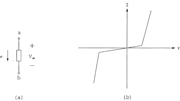
2.1 (a) Representation of a two-terminal nonlinear device; (b) i-v characteristics of a two-terminal nonlinear device... 8

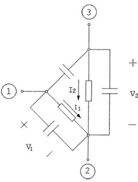
2.2 Representation of a three-terminal nonlinear device. 9

5.1 RLC underdamped circuit with real and complex poles. 30

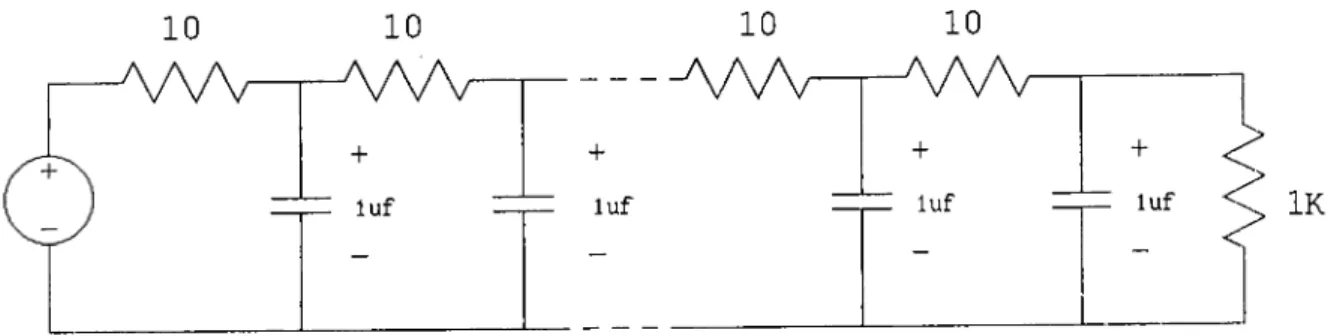
5.2 RC tree with a length of 10. 31

5.3 First order approximation to the response at the end of the

tree. 32

5.4 14*^ order RLC ladder.

5.5 Transient simulation of the 14*^ order RLC ladder.

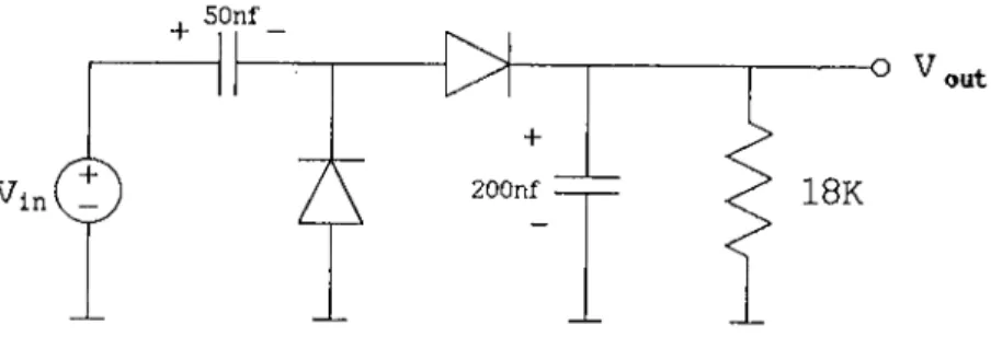
5.6 Voltage Doubler Circuit.

5.7 Transient analysis of the voltage doubler.

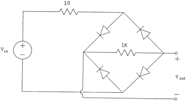
5.8 The circuit of the full-wave rectifier.

5.9 Transient analysis of the bridge rectifier.

5.10 CMOS Inverter.

5.11 Model of the M OSFET’s used in CMOS inverter.

33 33 34 34 35 36 36 37

5.12 The result of transient analysis of the CMOS inverter, and the

operating segments of the transistors. 38

5.13 The circuit of CMOS NAND Gate. 39

5.14 The result of the transient analysis of the CMOS NAND Gate. 40

5.15 Operating segments of the transistors in the CMOS NAND

Gate. 41

5.16 The circuit o f CMOS Logic Function Unit.

5.17 Transient respon.se of the CMOS Logic Function Unit.

42

List of Tables

5.1 Approximate Poles for response at. C2 and the actual poles of

the circuit. 30

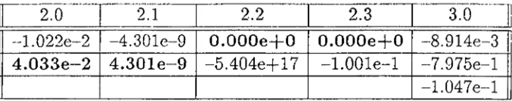
5.2 Trials of BUSTLE to find a second order approximation to L3 and conclusion with a third order approximation. 30

INTRODUCTION

In circuit analysis and design, various circuit simulation tools are used based on different requirements of accuracy and execution speed. These require­ ments depend on the type and size of the circuit which is to be simulated. As expected in any numerical simulation there is a trade-off between the accuracy and speed of program execution. As the device sizes get smaller and smaller, and the number of devices in a system increases, this trade-off becomes a bottleneck in simulation of circuits, especially for VLSI circuits.

The complex nonlinear characteristic of devices and the large number of iterations needed for computing the transient response in timing simulations result in extensive computations and thus very long simulation time. Al­ most all of the circuit simulators use numerical and iterative methods (e.g. Newton-Raphson) to handle nonlinear characteristics and numerical integra­ tion methods (e.g. Forward Euler, Backward Euler, Trapezoidal, etc.) to compute the transient response of energy storage elements.

An important point for a simulator is that it should be adaptive to new devices resulting from the emerging technology, in order to prevent it from being obsolete in a short time. Even the user must have the capability of doing this integration.

By the motivation of the^above facts, ■'a new circtnt simulation tool, BUS- TLE (Bilkent University Simulation T ool for Linearized Environment) is developed. Our first aim is to terminate the simulation by success (no con­ vergence problem). Instead of numerical integration methods, Asymptotic Waveform Evaluation (AWE) technique is employed in BUSTLE to compute the response of energy storage elements.

CHAPTER 1. INTRODUCTION

One of our major goals is to finish the job in a reasonably short time. To achieve this, Piece-wise-linear (PW L) approadi is used to characterize the nonlinear elements. The main reason behind our choice of PWL approxi­ mation is that it deals with a set of linear equations and avoids solving of nonlinear equations. As a result of this, time complexity is decreased and the convergence in DC Analysis is guaranteed. Furthermore, AWE is mainly for linear(ized) circuits. Therefore, the use of PW L approximation makes the utilization of AWE easy and efficient for nonlinear devices.

Another important reason for choosing the PW L approximation is flexi­ bility so that the user can easily define his own device models for nonlinear devices. Subsequently, it provides the user to make an optimal trade-off be­ tween the accuracy and the speed of the simulation. This makes the simulator independent from the technology.

Using AWE, transient analysis is the part that needs the most attention. Since we find the approximate poles and the residues for any output of the circuit, only a simple plotting routine does the AC analysis. A D C analysis is already performed prior to the transient analysis to find the operating points of the circuit. The sensitivity analysis using AWE technique may also be handled with a little additional cost [5,25].

This project was done in collaboration with M. Murat Alaybeyi and Satılmış Topçu. The work related to Asymptotic Waveform Evaluation be­ longs to myself. The sparse matrix solver routines [1] was written by M. Murat Alaybeyi. DC Analysis part was constructed by M. Murat Alaybeyi and myself. The work for Transient Analysis was also carried out by M. Mu­ rat Alaybeyi, Satılmış Topçu and myself. We have implemented BUSTLE, in the C Programming language on SUN-3/60 and SUN-3/110 Workstations running under the UNIX operating system.

The organization of the thesis is as follows: Chapter 2 explains the form of network equations, the solution method to solve the network equations, (LU decomposition), PWL modeling of nonlinear devices and the algorithm used in finding the operating points for the nonlinear circuits. Chapter 3 focuses on the Asymptotic Waveform Evaluation. It includes theoretical background for AWE and introduces the Derivative Moment concept and the Moment Shift­

ing algorithm to handle the unstability problem of AWfi. It also explains the

computation of derivative and integral moments and^<^w to handle the loops and cutsets of energy storage elements. Chapter 4 describes the method of transient analysis using AWE and PWL devices. Some implementation issues

of the transient analysis are also mentioned in this chapter. In Chapter 5, illustrative examples are provided for a variety of circuits and the simulation results are compared with SPICE. Conclusions are in Chapter 6. In addi­ tion, BUSTLE User’s Guide is supplied in the Appendix part with several examples.

Chapter 2

DC ANALYSIS

Finding the “operating point” or “DC solution” of a network is usually the first step in the analysis of nonlinear networks. It involves determining the node voltages for given values of DC sources and is equivalent to the solution of nonlinear algebraic systems of equations. In this work, piece-wise linear (PW L) representation is used to characterize the nonlinear elements. There­ fore, the nonlinear network is replaced by a piecewise-linear network with a corresponding simplification of the problem. Consequently, solution of non­ linear algebraic systems of equations are reduced to the solution of a set of linear systems of equations.

M X = b (2.1)

where M is the matrix that describes the resistive network, and b is the source vector.

2.1

Network Equations

Kirchhoff current law (KCL), Kirchhoff voltage law (KVL) and the element constitutive equations (CE) are used to describe a resistive linear network. There are three general methods to formulate network equations. Nodal for­

mulation, Mesh formulation and Tableau formulation [26].

Nodal admittance formulation is based on the Kirchhoff current law which states: The algebraic sum of currents leaving any node is zero.

Y V = J (

2

2

where Y is the nodal admittance matrix, J is the current source vector, cUid V is the vector containing node voltages, to be solved for.

The mesh formulation is similar to the nodal formulation and is useful in hand calculations on simple networks. The basis for the mesh formulation is the Kirchhoff voltage law: The sum of voltage drops around any loop is zero.

Z I = E (2.3)

where Z is the branch impedance matrix, E is the voltage source vector, and I is the vector containing branch currents.

These two formulation methods are quite efficient and have been used successfully in many applications, but they can not handle all idecil elements. To avoid restrictions. Tableau Analysis Method is used for the formulation of network equations [26]. In Tableau Analysis Method, all equations describing the network are collected into one large matrix equation, involving the KCL, KVL, and the constitutive equations. KCL can be expressed by

A lb = 0

whereas the KVL is given by

V , - = 0

(2.4)

(2.5) where A is the incidence matrix [29], Ib is the vector containing branch cur­ rents, Vb and ~Vn are the brancli and node voltages respectively.

Branch constitutive equations can be written as

G Vb + R Ib - w (

2

6

where w is the vector including the independent current and voltage sources, as well as the influence of initial conditions on capacitors and inductors. This vector also includes the equivalent sources due to linearization of nonlinear elements.

Equations (2.4)-(2.6) can be put into one matrix equation.

(2.7)

' I 0 -A ^ ’ ‘ ■ Vb ■ ’ 0 '

0 A 0 _R 0

G R 0 _{. V - .} w

M

Some advantages of Sparse Tableau Analysis is that, partitioning of M matrix is straightforward in this type of formulation. And all brancli voltages, branch currents cind node voltages are comi^uted by solving the equation

CHAPTER 2. D C ANALYSIS

(2.7). But in the Nodal analysis, only the node voltages are calculated, branch voltages and branch currents should be computed separately resulting in more complicated programs.

On the other hand, the resulting matrices are always quite large in Tableau formulation. But these matrices are more sparse than the ones in the Nodal formulation. However, if a good sparse matrix solver routine is available, then the efficiency becomes better than the Nodal analysis.

2.2

LU Decomposition

In network applications, the solution of algebraic equations is best performed by the triangular decomposition or LU factorization technique [26]. Algo­ rithms for triangular decomposition are closely related to Gaussian elimina­ tion, though the computations might be performed in a different sequence. The main advantage of triangular decomposition over Gaussian elimination is that it enables simple solution of systems with different right-hand-side vectors.

Let the systems of equations be given by (2.1) and assume that the matrix M can be factored as follows:

M = L U (

2

8

where L is a lower triangular matrix and U is a an an upper triangular matrix. Then the systems of equations can be rewritten as follows:

Define an cuixiliary vector z as

L U x =

b

U x

(2.9)

( 2,10)

At this time, z can not be calculated because x is unknown. However, sub­ stituting z into (2.9) we get

L z = b (2.11)

Due to the special form of L, the vector z can be calculated very sirnplj^. This is called forward elimination or substitution process. Since we know z, agciin equation (2.10) can be calculated very easily due to the special form of U. This process is called backward substitution.

Thus, once we LU factor the M matrix, then solving equation (2.1) be­ comes very easy and fast for different

b

substitution (FBS). So, the main task in solving the equation (2.1) is the LU factorization of the M matrix.

As we said before, the M matrix is very sparse which means most of the elements of the M matrix is zero. One can save a lot of operations by not performing the multiplications and additions on these zeros. In fact, the zeros need not even be stored, thus reducing the memory requirements.

A sparse matrix algorithm is used in BUSTLE to solve the network equa­ tions. The M matrix is stored in a suitable structure to make the LU fac­ torization efficient and fast. The detailed information on the data structure and the algorithm for LU factorization is described in [1].

2.3

Modeling of Nonlinear Devices

Modeling is the process by which the electrical properties of a semiconductor device is represented by means of mathematical equations or tables. Physical device models usually involve many complicated equations. Typical timing studies have shown that the major part of the computational effort in network analysis is spent in evaluating these complicated relationships. Further, most analysis methods also require derivatives of the model equations, which is a cumbersome and error-prone task for the designer. The iterative methods, such as Newton-Raphson, to solve the nonlinear equations do not guarantee the convergence. In order to avoid these problems, piece-wise linear approach is used in BUSTLE for the modeling of nonlinear devices. It should be recognized that if a kirge number of sample points-are selected to define a nonlinecU' characteristics, the description approaclies that of a continuous function. But in this case the execution time may be very long. Table models are employed to describe two and three terminal nonlinear devices.

2.3.1

Modeling of two-terminal nonlinear devices

The i-v characteristics of two-terminal nonlinear devices are defined by the sample i-v values extracted from the nonlinear characteristics. BUSTLE assumes that the i-v characteristics is linear between these points. By using these values, the resistance Ri, the conductance G'/, and the equivalent source

CHAPTER 2. DC ANALYSIS iiJù + Ô b (a) (b)

Figure 2.1: (a) Representation of a two-terminal nonlinear device; (h) i-v characteristics of a two-terminal nonlinear device.

wi due to linearization, of a two-terminal nonlinear device can be calculated

very easily.

In the tableau formulation, the nonlinear elements may be either volta.ge or current controlled. Both cair be implemented by their piece-wise linear approximation. Note that in the segmeirt having the slope Gi (for the voltage-controlled case), or Ri (for the current-controlled case) there is an additional source or respectively coming from the linearization of the nonlinear devices. The equations for the element in the segment are

Î — T Giv

V = v f + Rp

and, in general.

G; V/, + R / l6 -- W/ The tableau equations can be written as follows:

(2.12) (2.13) I 0 G, or in compact form 0 -A'^' A 0 R/ 0 ■ Vfc ■ 0 ’ 0 ’ l6 0 + 0 W/ w (2.14) M/ X; = W; -f W (2.15)

©

+

V2

Figure 2.2: Representation of a three-terminal nonlinear device.

The subscript I denotes the segment in which the network operates. The right-hand-side vectors, W / and w denote the equivalent sources due to lin- eariza,tion and the independent sources, respectively; they are written sepa­ rately for clarity.

2.3.2

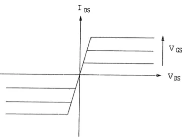
Modeling of three-terminal nonlinear devices

Three-terminal nonlinear devices are represented as a combination of two 2- terminal device placed between the three nodes as shown in Figure 2.2. There is no need to place another 2-terminal device between the nodes 1 and 3 since its voltage and current are also defined by the other two due to KVL and KCL. The parasitic capacitors are also included in the device model. The values of these capacitors are given in the model card.

The characteristics of a three-terminal nonlinear device is defined by two equations and a number of boundaries for each region. These two equations define an hyi^erplane in the 4-dimensional space which describes the i-v char­ acteristics of the nonlinear device where the boundaries describe the region at which these equations are valid. The branch equations for the three-terminal nonlinear devices are of the form:

CHAPTER 2. D C ANALYSIS 10

and at most three of the coefficients 01,02, 03,04 can be nonzero since one of them can be eliminated using the other brandi equation. The boundaries are described by the inequalities of the following form.

OiUi + O2U2 + 03^1 + 04^2 + O5 > 0 (2.17) and at most two of the coefficients oi, 02,03,04 can be nonzero since they have to satisfy the two branch equations, two of the variables can be eliminated. Each nonlinear device must contain a segment that satisfies the origin (both the equations and the bouncUiries) in order to have a valid solution when all of the independent sources are killed. This is required in order to start the DC analysis which will be described in the next section. The coefficients of the branch equations, which a.re called stencils, directly contribute the M matrix given in equation (2.14) and (2.15). Note that this modeling scheme does not introduce any restriction to the user defined model approach.

2.4

D C Analysis: Finding the Operating Point for Non­

linear Devices

The solutions to a circuit with DC inputs are called operating points. The term D C Analysis refers to the determination of operating points. For DC solution, all inductors are short-circuited and all capacitors are removed from the circuit. Given a valid solution Xq for an arbitrarj^ source vector yo and satisfying the boundaries of the region Rq,

Mo xo = Wo + yo (2.18)

we would like to find the solution x and the region R f for a given source vector y.

M / X = w / d- y (2.19)

The algorithm used in the DC Analysis has been derived from the Kaizenel-

son’s algorithm [8,9] which guarantees the convergence in the DC Analysis

[7], The modified version of the Katzenelson’s algorithm, used to find the solution X and the final operating region set R j, is as follows:

1. Set i = 0. 2. Solve X from

3. If X satisfies the boundaries of R{ then TERMINATE, else GOTO 4. 4. Let A be the ratio of the distance from x, to the first region boundary-

crossed -when traversing from Xi to x, to the distance from x,· to x. 5. Compute Xi+i as

Xi+i = X,· + A(x - Xi).

6. Set to the neighbor region of 7?,· separated from it -with the first crossed boundary.

7. Increment i and GOTO 2.

Note that for the first DC analysis, Xo and yo can be selected as 0, since by definition, every nonlinear element is modeled to have a passive resistive segment satisfying the origin, and that satisfies the solution -when all the sources are killed. It is obviously a poor starting point, but that is the only valid solution kno-wn initially. Afterwards solutions of the last DC analysis are chosen as Xq, yo, and Rq. It is expected to do fewer calculations starting from the last solution, since it is more probable that the old solution is closer to the new one than the origin (0).

Chapter 3

ASYM PTO TIC WAVEFORM

EVALUATION

AWE is a recent technique for the approximation of linear, time-invariant circuits [2,3]. It is, in fact, a form of Fade approximation [10,11,12,14,15]. The main idea in AWE is that, the response of energy storage elements, which require the use of numerical integration methods, is approximated, by using the method of moment matching and domina.nt pole-zero approximation. Analytic expressions for the response of energy storage elements are obtained using the AWE technique. Then these expressions are evaluated and used to solve the rest of the circuit.

3.1

Theoretical Background

AWE is explained in detail elsewhere [3,2]. We summarize it here for com­ pleteness and also to establish the slightly different notation.

AWE is most conveniently explained, in general, in terms of the differential state equations for a lumped, linear, time-invariant circuit:

X = A x -(- Bu, x(0 ) = X() (3.1)

where x is the n-dimensional state vector and u is the m-dimensional input vector. Such a circuit description can be found for all circuits.

This equation (3.1) has a well known solution. But for large circuits, the matrices A and B becomes so large that, it becomes practically impossible to solve this equation. Instead, a suitable approximation for Xi is sufficiently

good for our purposes, where X( is the state variable in x. Our aim is to find such an approximation.

Suppose that the particular input Up(i) is of the form:

Up(t) = Uo + Ui:i, f o r t > t o , (3.2) where Uq and Ui are constant m-dimensional vectors. This corresponds to a step plus ramp type of input. In general, the input Up{t) is not restricted to such simple signals, but rather could assume any form of input for which a particular solution can easily be obtained. The particular solution of the differential state equation (3.1) corresponding to Up(i) in Eq. 3.2 is:

^Buo — A ^Bui — A (3.3)

Matrix A should not be singular for the particular solution to exist. This condition is equivalent to specifying that the circuit has a unique and well- defined DC solution (when all of the capacitors are open-circuited and induc­ tors short-circuited, the M matrix in equation (2.7) must be non-.singular). Finding a particular solution to a more general and complex input such as:

(3.4)

Up(t) = sin(c-.;pt + f)

is only algebraic manipulation.

That leaves us with the task of obtaining the homogeneous solution

Xh = Ax/, (3.5)

for which we must alter the initial conditions to compensate for those of the particular solution. The initial condition for the homogeneous equation (3.5) is:

x/i(0) = xo + A ~ ^ B u o-f A “ ^Bui (3.6) where Xq is the initial conditions at time zero. One way of solving the homo­ geneous equation (3.5) is to use the Laplace Transform.

X ,(s ) = ( s l - A ) - ^ x , ( 0 ) (3.7)

If the Laplace Transform of the homogeneous equation (3.7) is expanded using the Taylor Series expansion around s = 0, we get:

CHAPTER 3. ASYM PTO TIC WAVEFORM EVALUATION 14

Using the definition of Laplace transform and the Taylor Series expansion around s = 0,

Xfc(-s) =

f

where m -k is the moment ^ and particularly called the integral mo­ ment. Now, if the two series in the equations (3.8) and (3.10) are matched term by term, we get the relationships,

m _i = -A -^ x /j(0)

m_2 = -A ~^x;,(0) = A~^m_i m_3 = -A ~ ^ x/i(0) = A "^ m_2

m_2,+i = - A ^’ +^x/i(0) = A ^m_

(3.11)

And the initial condition may be represented as the zero-th moment ^ , n io , to establish a recursive relationship.

nio = -x ;i(0 ) (3.12)

Then we can summarize the equations in (3.11) by the simple recursive rela­ tionship

niyfe-i = A'^m^:, fo r k < 0 (3.13)

Let us pick, in particular, the state variable and focus on the com­ ponent of all moment vectors. We can make a order {q < n, typically

q n, where n is the order of the circuit) transient approximation to the

solution of the state variable by matching their 2q moments coming from the equations (3.11) and (3.12).

1=1

(3.14)

^Note that, our notation is slightly diiTerent from the notation used in [2,3]. If the equation (3.10) is rewritten according to their notation, it becomes

oo X/l(«) =

it=0

The reason for the diiTerent notation is to combine the derivative moments, which will be explained in the next section, w.ith these moments easily.

^According to the notation o f [2,3], initial condition is represented by the (-1)^^'' moment,

In equation (3.14), p/’s and ki’s are the complex approximating poles and their corresponding residues, respectively. There are 2q unknowns in Eq. 3.14, where q of them are the poles and the remaining q are their corresponding residues. We should be able to solve them from the 2q equations, which comes from the moments.

If we take the' Laplace Transform of (3.14) and use the Taylor Series expansion around s = 0 again, we get:

Y f ^ kt/pi /=1 ^ Pi

’ k

E

Again, if the coefficients of the s terms in the equations (3.10) and (3.15) are matched, we get the following set of equations for the state variable upon inclusion of the initial conditions

— + A:2 + ^3 + ■ ■ ■ + kq) — [iTio],·

= [m-l],·

= [m-2

],·

2

where [m_fc]^’s are the moments corresponding to state variable. Under the assumption that the moments can be calculated easily, without much of a computational cost, we have 2q equations. We merely need to solve

2q unknowns, which are the approximating poles and their corresponding

residues. Unfortunately, these 2q equations (3.16) are nonlinear. One can attempt to solve these equations using iterative methods such as Newton- Raphson. Instead, we will try to reformulate the problem to allow for the direct solution of the approximating poles and residues. If we summarize the set of nonlinear equations given in (3.16) in matrix form such as

- V k = ¡m jj ■ V p -«k = [ m jj

(3.17) (3.18) where [nii],. and [m/i],· are the low^order and high-order moments of the f'* state variable, respectively. P is a diagonal matrix that contains the poles at

CHAPTER 3. ASYM PTO TIC WAVEFORM EVALUATION 16

the diagonals and V is the well-known Vandermonde Matrix [21,22] and k is the vector of residues corresponding to state variable.

[m_,+a]. ] (3.19) (3.20) V = k = [n^o],· [1^ -1].· [m_2],. ·· [

111

If the equations (3.17) and (3.18) are rewritten, we get the following relationships.

k = -V-^m,

and

V P - ’ V - 'm , = m;, (3.24)

Since the Vandermonde Matrix is a modal matrix for a system in companion form [26], equation (3.24) is equivalent to

A j ’ ni/ = m/i (3.25) where

A. =

0

0

ao —cii —a2 · * · —a^-i

(3.26)

The characteristic equation that goes with the original order homoge­ neous equation is

4" cLiX “h ci2^^ 4" * * * 4" ciq-iX^ ^ 4" = 0 (3.27) If Ac is recursively applied to ni/, then equation (3.25) can be rewritten to yield the following result, [3].

mo

_{9 + 1}

where m _j is the integral moment of the state variable. If the above equation (3.28) is solved for a^s, then we can form the polynomial in equation (3.29).

aop’ + ^--- l· + 1 = 0 (3.29)

The roots of the q’th order polynomial above are the poles of the iY'’ state variable. And the corresponding residues can be computed using the equation (3.23).

Now, we know the approximating poles and the residues of the state variable, then response of that state variable can be calculated using equation (3.14). Note that, if the approximating poles are not distinct, then the Van­ dermonde Matrix becomes singular and the equation (3.23) has no unique solution. In this case, the Vandermonde Matrix has the form

V = 0 P' P' ,- 2 - p

—2p~^

2p-3

P

( - q + i)p

’ (-g)(-<z + i)p ’

^

As it is seen, second column is the derivative of the first one, and the third column is the derivative of the second one, etc.

If we summarize, determining the set of q approximating poles and residues, which are the dominant poles and their corresponding residues, requires: solv­ ing a q^^ order linear equations (3.28), then solving the roots of the ch.arac- teristic polynomial (3.29) which is, again, q^^ order.

3.2

A W E Using Derivative Moments

We have presented the moment concept in the previous section. Remember that the moment is the integral of i^'x/i(i) from f = 0 to oo (3.9). From no\v on, we will call the moments given in terms of the equation (3.9) and (3.10) as integral moments. Integral moments give information about the integra.1 of the actual response. They correspond to the coefficients of the Taylor series expansion of the Laplace Transform of the original response around s = 0. Although AWE can find good approximations using integral moments, in some cases, we need the derivative of the actual response also. This necessity arises from the fact that, AWE may not find stable approximations which

CHAPTER 3. ASYM PTO TIC WAVEFORM EVALUATION 18

will be explained in the next section. In these cases, derivative information may be used to overcome this difficulty. Derivative moments can be described similar to the integral ones by using the recursive relationship.

m i = - A x * ( 0 ) = Amo

ni2 = A m i

m

3

2

m2,_i = A m2g_2.

where X/,(0) is again given by the equation (3.6).

(3.31)

The approximating poles and their corresponding residues can be calcu­ lated using the same method described in the previous section. If we sum­ marize, the coefficients of the characteristic polynomial are calculated from equation (3.32).

mo mi

mi

m2

where mj is the derivative moment of the state variable. And the approximating poles are the reciprocals of the roots of the i)olynomial given in equation (3.33).

ooP® + oip^ ^ + 02p’

H

---l· a,_ip -f 1 = 0

The corresponding residues are calculated using the equation (3.23), where V and m; are given by

V = 1 1 1 Pi P2 _P<! (3 .3 4 ) ? - l Pi p r ’ _ [mo]i [mi],· [ n i ,- i ] i r (3 .3 5 )

where pi’s are the reciprocals of the roots of the polynomial given in equation (3.33). Note that, the Vandermonde Matrix in this case is slightly different from the previous one. Also, poles are the reciprocals of the roots of the equation (3.33), instead of the simple roots of the equation (3.29). But if we

use the zeros of equation (3.33) to construct the Vandermonde matrix, then the two methods will be identical, except l / p , ’s should be used in equation

(3.14).

Consequently, we can also perform the AWE using derivative moments. Derivative moments correspond to the coefficients of the Taylor series ex­ pansion of the Laplcice Transform of the original response around .s = oo. Therefore, using derivative moments in AWE may give better results in tran­ sient analysis. Furthermore,using the combination of derivative and integral moments also helps us get rid of the unstability pi’oblem in AWE.

3.3

A W E Using the Combination of the Derivative and

Integral Moments

Using AWE, we may find unstable approximations for stable circuits. This is because, we are trying to approximate a higher order system with a lower order one. And moments can give inconsistent information for that lower order system. For example, assume that the original waveform has a nega­ tive initial condition and goes to zero at steadj'· state after a large positive overshoot in the initial part of the response (i.e. the area under the original response is positive). If we use the integral moments for matching, the first order approximation can not find a stable pole. Because we are trying to fit a decaying exponential, starting from a negative value (initial condition), but with a positive integral from 0 to oo, which is obviously not possible. But, if we use the first derivative moment approximation or a second order approximation (derivative or integral or a combination of both), we can find a stable approximation. We may also end up with RHP poles using only the derivative moments. So it is a good idea to use different combinations of integral and derivative moments, for calculation of poles and residues of every state variable independently.

If we rewrite the equations for both derivative and integral moments.

nio = - -X/i(0)

m _i = A~bno n il = Anio

m_2 ni2 = A m i

CHAPTER 3. A SYM PTO TIC WAVEFORM EVALUATION 20

Notation is such that, integral moments have negative indices where the derivative moments have positive, and mo matches the initial conditions.

Now, we have Aq moments, 2q of them among all, are the derivative moments whereas the remaining 2q are integral moments. One needs 2q moments, including the initial condition mo, to solve the approximating poles and corresponding residues. The remaining (2q — 1) moments may contain any number of derivatives, or integrals.

We have seen two similar methods to calculate the poles and residues. One uses the integral moments, where the other uses the derivative moments. Any of the two methods may be used for the calculation of poles and residues. But it is easier to use the method which uses the integral moments when the number of integral moments used in the approximation is greater than the derivative moments, and the other method when the number of derivatives is greater.

Now, let’s see the form of equations when the combination of derivative and integral moments is used.

i) When the number of integral rn,oments > the number of derivative mo­ ments.

Let s be the number of derivative moments which is used in the q^’'· order approximation. Then the moment equation (3.28) is modified such that

m , rris-x rris-i rUs-i ms -q + l Oo rris-q « 1 '^^s— q — 1 Ctq — l '^^s — 2q+i (3.37)

where mj is the integral moment if j is negative, or the derivative moment if j is positive, for the i*^ state variable. And the poles are the roots of the polynomial given in equation (3.29). The residues are calculated again by using the equation (3.23) where V and m; are given by the equations (3.19) and (3.21) respectively.

ii) When the number of derivative moments > the num,ber of integral moments.

Let again s be the number of derivative moments which is used in the

that m _ · m-s+i m-s+i Tn^s-\-q — l ao ^-54-7 ai = — (3.38) m-s+g · • · m^S‘\-2q-2 ^q — l m^s+2q-l

where again mj is the integral moment if j is negative, or the derivative moment if j is positive, for the state variable. The poles are the reciprocals of the zeros of the polynomial given in equation (3.33). The residues are calculated by using the equation (3.23) where V and ni; are given by the equations (3.35) and (3.34) respectively.

Consequently, we can use any number of derivative moments in AWE to compute the poles and their corresponding residues by using the methods described above. This also helps us find stable approximations in AWE.

3.4

Moment Shifting Algorithm

The number of derivative moments is an important parameter in AWE. As it is mentioned before, AWE may not always find stable api.)roximations. In such cases, one solution is to increase the order of approximation, b\it some examples have shown that this may not work, due to numerical inaccuracy which occurs when the order of approximation is high. The numerical in­ accuracy arises from the moment matrix in equation (3.28) which becomes ill-conditioned when the approximation order increases. An interesting “rule of thumb” is given in [19] regarding the numerical limitations of Fade ap­ proximation: The highest order of denominator in a Fade approximation is about one fourth of the number of bits used in the mantissa of the computer’s floating point representation. Since AWE is a form of Fade approximation, it also suffers from such limitations. Many approaches have been proposed to circumvent the unstability problem of Fade approximation [13,16,17,18]. But the computational complexity of those methods are not reasonable. However, unstability problem may be overcome by using different number of derivative moments in the approximation without increasing the order.

CHAPTER 3. ASYM PTO TIC WAVEFORM EVALUATION 22

• Necessary moments are computed according to the order of approxima­ tion.

• For every state variable DO

(i) Compute the poles using the proper moments (initially start from all integral moments if the user does not redefine this parameter). (ii) If there is any unstable pole then

If there are no integral moments used then increase the order of approximation by 1, else

replace the highest order integral moment with the next derivative moment, and go to (i) to compute the poles. (iii) Compute the residues.

So, the number of derivative moments used in the approximation is in­ creased one by one until a stable approximation is found or all of the integral moments are replaced with the derivative ones. If a stable approximation can not be found then the order of approximation is increased by one. And we are trying to avoid large orders, due to numerical errors and increased number of operations which consumes long time for approximation. But we have observed for a large number of examples that a stable and good approx­ imation can be found below the 5’th order. If a stable approximation can not be found up to a certain order, (which never occurred for all the excimples we tried) the order of approximation is not increased anymore, but the first derivative (Forward Euler) is used to approximate the response to shift in time. Afterwards, a new AWE is made with different initial conditions. Note that the dominant approximate poles and residues depend on the initial con­ ditions. Also note that, using this algorithm, the order of approximation and the number of derivative moments used in the approximation may not be the same for different state variables. And it is not necessary to approximate all of the states with the same order for transient analysis as far as one can find a good approximation for that state variable.

3.5

Computation of the Derivative and Integral M o­

ments

Moments are defined by the recursive relationship given in equation (3.36). We know that mo matches the initial conditions. Therefore it is easy to

compute nio first. Then, derivative and integral moments can be computed by recursively multiplying it with A and respectively.

In order to compute nio, we need to find the particular solution, Xp(i) in equation (3.3), corresponding to the particular input, Up(i) in equation (3.2). The term A~^Buo in the X p ( i ) , is the steady-state (i.e., capacitors open circuited, inductors short circuited) solution of the circuit with the input Uq. The term A “ ^Bui again corresponds to the steady-state solution of the circuit with the input Ui. And the term A “ ^Bui is calculated by multqfiying A "^ B u i with A ’ as described in the computation of integral moments.

After the computation of mo, we can compute the derivative and integral moments. In order to compute the integral moments, we must multiply the m/c with A “ ^. To do this, we kill all the input sources, i.e. we set u = 0. Assuming there are no loops of capacitors and cut-sets of inductors, replace all capacitors with current sources of value (C x m^) and all inductors with voltage sources of value (L x mk), where C and L are the capacitance and inductance values respectively, and rn.k is the integral moment for the corresponding state variable. Then, the voltages across the current sources (replacing the capacitors) and currents through the voltage sources (replacing the inductors) are the next integral moments.

In order to find the derivative moments, all the input sources are killed. We replace all capacitors with voltage sources and all inductors with current sources of value m/,, where mk is the derivative moment for the corre­ sponding state variable. Then, the currents through the voltage sources (re­ placing the capacitors) and the voltages across the current sources (replacing the inductors) are X A m ^ , where

X = C

0 0

L (3.39)

Then, we can compute Am^, which equals to nir+i, by multiplying the above term by X " h

Thus, we carr compute the derivative aird the integral moments by using the above recursive algorithms. Note that the computation of moments does not involve LU factorization, but a simple forward and backward substitution (FBS) for each moment.

X is a diagonal matrix if there are no loops of capacitors and and cutsets of inductors. Handling of capacitor loops and inductor cutsets will be described in the next section. Therefore the matrix X remains diagonal, thus the

CHAPTER 3. ASYM PTO TIC WAVEFORM EVALUATION 24

multiplication by X ^ does not involve matrix inversion or LU fe.ctorization of X matrix but just a division by a floating point number.

3.6

Loops and Cutsets of Energy Storage Elements

In solving for the derivative moments or during the calculation o f the tran­ sient response of a circuit, every capacitor is converted to a voltage soiirce. Naturally loops of capacitors result in redundancy in the circuit equations.

BUSTLE handles this situation by first constructing a proper tree [20]. The capacitors in the tree are converted to voltage sources. The capacitors in the co-tree will form loops with tree capacitors. The voltages across the co-tree capacitors are determined by the tree capacitors. Therefore, we need to put some constraints on the currents around the loop, for a proper current distribution [4]. Let us think about a capacitor loop, with n capacitors,

C i,C2·, ■ ■ · iCn·, oi which Cn has been determined to be in the co-tree, and the

others in the tree, it comes from the KVL that

vc„ = v c , +VC2 + --- h (3.40) If the derivatives of the both sides are taken with respect to time, we get

(3.41)

(3.42)

dt dt dt dt

Equation (3.41) can be rewritten as

Cn C , C 2 ■■■ '

Equation (3.42) defines a current controlled current souree for C„ with the controlling branches {Ci^C^·, · · · , C„_i). Consequently, Cn can be replaced by a current controlled current source with the branch equation given in (3.42) which removes the redundancy in the circuit equations.

Similarly, cutsets of inductors cause a redundancy, when they are con­ verted to current sources. The same method can also be used for inductors. In this case, the inductor in the tree will i:)e changed to a voltage controlled

voltage source with the branch equation ‘^Ln

Tn

. ' ^ ¿ 2 I

+

Ln-i (3.43)

As a result, the equations corresponding to a co-tree capacitor and a tree inductor in the circuit equations are changed, redefining them as current

A similar problem exists for capacitor cutset, and inductor loops, which cause redundancies in the DC circuit equations. But this can be eliminated by using charge and flux conservations easily [6].

Chapter 4

TRANSIENT ANALYSIS

In transient analysis, BUSTLE computes the transient output variables as a function of time over a user specified time interval. In addition to the indepen­ dent DC sources, any independent source can be assigned a time-dependent value for transient analysis. Ideal step changes in the time-dependent sources are also handled without loss of generality. The transient respoirse is com­ puted using the AWE technique.

4.1

Transient Analysis Using A W E

A DC analysis is automatically performed prior to the transient analysis with the input values at time i = 0, in order to determine the operating segments/regions for the PW L devices and to calculate the initial conditions of the capacitors and inductors. If an initial condition is given for a capacitor voltage or an inductor current, these elements are replaced by voltage and cur­ rent sources respectively to force the initial conditions. Otherwise, inductors are shorted and capacitors are removed from the circuit. After determining the operating segments/regions for the PWL devices and initial conditions of energy storage elements, all inductors are replaced by short-circuits and all capacitors by open-circuits to calculate the steady state response, which is re­ quired for the computation of moments in AWE. The steady state response is calculated for step and ramp type of inputs separately. First, it is calculated by using only the step part of the inputs, then the slopes of the ramp inputs are used as sources to calculate the steady state response corresponding to ramp inputs. Then the response of a state variable, as a function of time.

can be written as follows.

?

~ ^SS,tep "b ^O.romp "b ^SSramp^ "b ^3 (4.1) ¿=0

where Xss„^p and Xssramp steady-state values corresponding to step and ramp type of inputs respectively, pds and /j,’s are the dominant poles and their corresponding residues, respectively, mo^ramp for the state variable is given as

mo,_{ramp A -^ x SSramp} (4.2)

The value of mo,ramp is calculated during the calculation of moments in AWE without an additional cost.

Once the dominant poles and the residues are calculated by AWE, we know the response of all energy storage elements by equation (4.1). Then all capacitors are replaced by voltage sources and all inductors by current sources of value given by the equation (4.1). By evaluating the equation (4.1) at certain time instants, we can solve the whole circuit by a. simple substitution to compute all voltages and currents in the circuit.

4.2

A W E with P W L Devices in Transient Analysis

Using AWE we obtain approximate analytic expressions for capacitor volt­ ages and inductor currents. These expressions are valid on the time axis as long as they satisfy the set of current operating regions iî,·. In order to find voltages and currents of each device, these expressions are evaluated at cer­ tain time instants by using these values as sources and the circuit is solved by a mere substitution. As we progress over time the nonlinear devices in the circuit may change their segments. If occurs, we must know the time when one nonlinear device, at least, changes its segment. As soon as we realize a segment change, we go back over time and search for the time of segment change. The capacitor voltages and inductor currents for that in­ stant of time are the initial conditions for a new DC analysis to find the new segments/regions for PW L devices. Then a new AWE is performed using the new segments/regions and the new initial conditions.

The same thing happens when there is an inj^ut change at time to. We evaluate the approximate expressions found for energy storage elements and solve the circuit at time Îq by a mere substitution. A new DC analysis is performed at time Îq using the new source vector, and a new AWE is

CHAPTER 4. TRANSIENT ANALYSIS 28

carried out for t > to. For DC analysis, we can use the previous solution and segments (instead of 0 vector) as the initial valid solution. Tiiis saves a lot of computation in DC analysis.

One problem about this algorithm is that, there is an inherent instability problem near the corners of the PWL elements, if the operating point is just on the corner. Although the algorithm is guaranteed to be convergent, the oscillations around the corner ¡Doint causes the simulation not to end in a feasible tirne. Even this situation occurs very rarely and in some specific examples, they are determined by some additional checks in the softwcire. If such a situation is realized, then we continue the analysis by assuming one of the segments for a while. This does not cause a large error since we are already near the corner.

4.3

Calculation of the Time-step in Transient Analysis

As it has been mentioned before, we progress over time by solving the circuit at certain time instants. The selection of the time step in transient anal­ ysis is a quite critical issue for the efficiency standpoint. If the time step is chosen too small, then too many unnecessary computations must be per­ formed. This may even cause the simulation not to terminate in a reasonable time. Conversely too large time steps may cause large errors if there exist high frequency poles with large residues. Another drawback of the large time step is that we may skip an overshoot of the waveform which may possibly cause a segment change. Therefore, the time step used in transient analysis is dynamically calculated after each FBS. In this calculation, we consider primarily the rate of change of the most rapidly changing exponential. The rate of change at time to is comi^uted by taking the derivative of equation (4.1) with respect to time at time to for all the state variables.

dx{t)

dt = XSSramp -t- (4.3)

t-to i=0

where k^s and p,’s are the complex residues and poles respectively for that state variable.

As a result of dynamic selection of the time step, the simulator spends more effort when there are rapid voltage or current changes, and progresses faster in the time axis if there are slow changes. This provides an event driven feature to the simulator.

RESULTS

In this chapter, we will present some results obtained by BUSTLE to demon­ strate its accuracy and efficieny. The program leaves the accuracy speed trade-off to the user by giving him/her a number of options. The minimum order of approximation which determines the number of moments matched in AWE is an important parameter for the accuracy of the approximation. For example, this parameter can be selected as one for a digital CMOS circuit, but this would not be sufficient for an RLC circuit that has an oscillatory response. The minimum order and also the number of derivatives that will be matched initially can be determined by the user. There are also some other parameters that can be set by rhe user to improve the accuracy or the speed. Another important feature is that, user can define his own models (or use the one from the library) for nonlinear devices. This provides a capability to keep pace with the emerging technology and user can control the accuracy speed trade-off by choosing the number of segments used for modeling.

All of the simulations are carried out in SUN-3/60 Workstcitions. And SPICE version 2G.6 is used to compare the results of BUSTLE both from accuracy and speed standpoint.

IL L U S T R A T IV E E X A M P L E S

The first example is taken from [3] to demonstrate the usage of derivative and integral moments together, to get stable approximations. If we use the basic AWE method [2,3], we end up with RHP poles for C2 and L3 for a second order approximation. However, using the method described in Section 3.4, we can find stable approximations for all of the state variables.

CHAPTERS. RESULTS 30

Rl 1 Ll IH K2 10 L2 IH R8 100 LS IH

u( t) (

^ V V\A- V V V—

;D

Figure 5.1: RLC underdamped circuit with real and complex poles.

2.0 2.1 3.0 3.1

-1.206e-2 -2.015e-2 5 .0 5 3 e - l -8.935e-3 3 .0 1 2 e -2 -1 .653 e+ l -1 .269 e-l —2.803c"f-0

-8.915e-3 -1.965e-l

4.0 5.0 Actual

-5 .556 e-l + j8.965e-l -1 .029 e-l -5.556e-l + j8.965e-l -5.556e-l - j8.965e-l -1 .330 e-l -5.556e-l - j8.965e-l

-8.914e-3 -8.914e-3 -8.915e-3

-1.023e-l -5 .556 e-l + j8.965e-l -1.029e-l -5 .556 e-l - j8.965e-l -9.797e+0

-9.998e+l

Table 5.1:. Approximate Poles for response at C2 and the actual poles of the circuit.

2.0 2.1 2.2 2.3 3.0 ]

-1.022e-2 -4.301e-9 O.OOOe+0 O.OOOe+0 -8.914e-3 4 .0 3 3 e -2 4 .3 0 1 e -9 -5.404e+17 -l.OOle-1 -7.975e-l -1.047e-l

Table 5.2: Trials of BUSTLE to find a second order approximation to L3 and conclusion with a third order approximation.

10 10 10 10 A A A ^ r A A A ^ ■ A A Aa - A A A / - 1 1 + + < r~ "n— luf — jr " n r~ > IK

Figure 5.2: RC tree with a length of 10.

Table 5.1 and 5.2 show the approximate poles ^ of C2 and L3, resj^ec- tively, for different approximation orders and different number of derivative moments used in the approximation. Notation is such that the first number in the column headers indicates the approximation order where the second indicates the number of derivative moments used in the approximation. As it can be seen from the Table 5.1 and 5.2, after using the first derivative moment, a stable approximation can be found for C2, whereas for L3 we can not get rid of RHP poles for the second order approximation even all combi­ nations of derivative and integral moments are used. In this case the order of approximation is increased automatically, and a stable approximation in the 3’rd order is found (Table 5.2). But the remaining states are approximated in second order which is the minimum required order. So, we are doing a better approximation for L3 which improves accuracy in addition to getting rid of the unstable poles. Similarly, after using the first derivative moment, a sta.ble approximation can be found in the third order for C2. The approximation is already stable in the fourth and fifth order without using any derivative moments. Note that, second and third order approximation are not sufficient to obsei've the complex poles of the response at C2. Since the RLC circuit is slightly underdamped there are two real poles closer to jio-axis than the complex conjugate pair, also the residues of the complex pair is small. V/ith such a pole configuration, the oscillatory response at capacitor C2 is not ob­ served until the order of approximation is 4 or greater. This is a natural consequence of the moment matching method which approximates the poles.

R C Tree w ith F in ite In p u t Rise T im e : F ig u re 5.2.

The second example is an RC tree which may be used as the model of an interconnect in a VLSI circuit. The order of the tree is 10. A transient analysis is performed using the first order approximation in AWE with a finite

CHAPTERS. RESULTS 32

Figure 5.3; First order approximation to the response at the end of the tree.

input rise time. The simulations are performed using SPICE and BUSTLE for the response at the end of the tree (Figure 5.3). Although the first order approximation is used for a order circuit, the results are almost the same. The normalized RMS difference between first order approximation and SPICE is 0.7%. Note that even the first order approximation is good enough for such a monotonie waveform. The required CPU time for the simulation of BUSTLE is 1.57 seconds, whereas it is 6.38 seconds for SPICE.

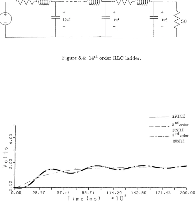
R L C lad d e r circu it: F ig u re 5.4.

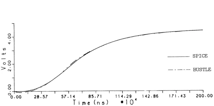
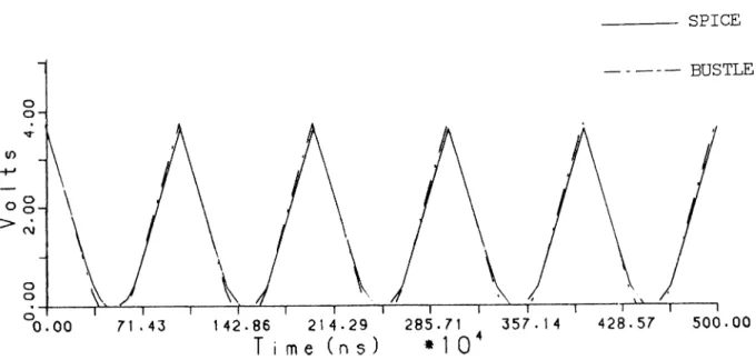
The third example is an 14*^* order RLC ladder. Transient analysis is per­ formed using second and third order approximation in AWE with a 3-volt ideal step input. The results of transient analysis at the end of the ladder, performed by SPICE and BUSTLE are shown in Figure 5.5. As it can be seen from the figure, BUSTLE 3'''^ order approximation and SPICE are in­ distinguishable from each other. However, the second-order AWE can not catch the oscillatory response. The normalized RMS difference between 2"'^ order approximation and SPICE is 2.99% whereas it is 0.35% in 3’·'·^ order AWE. The rec|uired CPU time for 2"^^ order approximation of BUSTLE is 2.1 seconds where it is 2.25 seconds for the 3’ ^^ order approximation. The CPU

/ / ; · ' » ' - X2( t) y dt N orm alized R M S d iffe r e n c e = u — — ---r—

10

^ v w - W

-luf luf ^

-50

Figure 5.4; order RLC ladder.

SPICE