Giil~en DemirSz and H. Altay Gfivenir
Department of Computer Engineering and Information Science Bilkent University, 06533 Ankara, Turkey
email: {demiroz, guvenir}@cs.bilkent.edu.tr
A b s t r a c t . A new classification algorithm called VFI (for Voting Fea- ture Intervals) is proposed. A concept is represented by a set of feature intervals on each feature dimension separately. Each feature participates in the classification by distributing real-valued votes among classes. The class receiving the highest vote is declared to be the predicted class. VFI is compared with the Naive Bayesian Classifier, which also considers each feature separately. Experiments on real-world datasets show that VFI achieves comparably and even better than NBC in terms of classi- fication accuracy. Moreover, VFI is faster than NBC on all datasets.
1 I n t r o d u c t i o n
Learning to classify objects has been one of the primary problems in machine learning. Bayesian classifier originating from work in recognition is a probabilistic a p p r o a c h to inductive learning. Bayesian approach to classification estimates the posterior probability that an instance belongs to a class, given the observed feature values for the instance. The highest estimated probability determines the classification. Naive Bayesian Classifier (NBC) is a fast, classical Bayesian classifier assuming independence of features. NBC has been found successful in terms of classification accuracy in m a n y domains, including medical diagnosis, compared with Assistant, which is an ID3-1ike [8] inductive learning system [5]. It has also been concluded that induction of decision trees is relatively slow as compared to NBC [5].
Considering each feature separately is common in both NBC, C F P (for Clas- sification by Feature Partitions) [3], and k-NNFP [1] classification algorithms. Both C F P and k-NNFP represent the knowledge as sets of projections of the training dataset on each feature dimension. K-NNFP stores all instances as their projections on each feature dimension, while C F P constructs disjoint segments of feature values on each feature dimension. The classification in C F P and k - N N F P is based on a majority voting done among individual predictions of features. The encouraging results and the advantages of the representation and voting schemes such as speed and handling missing feature values motivated us to come up with a new classification algorithm called the VFI (for Voting Feature Intervals). The concept is still represented as projections on each feature dimension separately, * This project is supported by TUBITAK (Scientific and Technical Research Council
but the basic unit of representation is a
feature interval
in VFI. Unlike segments in CFP, a feature interval can represent examples from a set of classes instead of a single class. The voting scheme, where a feature votes for one class, used both in C F P and k-NNFP, is also modified such that each feature distributes its vote among several classes.The voting scheme in VFI is analogical with the probability estimation in NBC. In NBC, each feature participates in the classification by assigning prob- ability values for each class and the final probability of a class is the product of individual probabilities measured on each feature. In VFI, each feature dis- tributes its vote among classes and the final vote of a class is the sum of all individual votes given the features. The results of the experiments show that VFI achieve comparably and even better than NBC on some real-world datasets and usually better than C F P and k-NNFP in terms of classification accuracy. Moreover, VFI has been shown to be faster than all other three classifiers, which suffer more on datasets having large number of instances a n d / o r features.
T h e next section will describe the VFI Mgorithm in detail. In Section 3, the complexity analysis and the empirical evaluation of VFI and NBC are presented. Finally, Section 4 concludes with some remarks and plans for future work.
2
T h e V F I A l g o r i t h m
This section describes the VF[ classification algorithm in detail. First, a descrip- tion of VFI is given. Then, the algorithm is explained on an example dataset.
2.1 D e s c r i p t i o n o f t h e A l g o r i t h m
The VFI algorithm is a non-incremental classification algorithm. Each training example is represented as a vector of feature values plus a label that represents the class of the example. From the training examples, VFI constructs feature intervals for each feature. The term
interval
is used for feature intervals through- out the paper. An interval represents a set of values of a given feature, where the same subset of class values are observed. Two neighboring intervals contain different sets of classes.The training process in the VFI algorithm is given in Figure 1. T h e procedure
find_end_points( Training,get, f, c)
finds the lowest and the highest values for linearfeature f f r o m the examples of class c and each observed value for nominal feature f f r o m the examples in
TrainingSet.
For each linear feature 2k values are found, where/r is the number of classes. Then the list of 2k end-points is sorted and each consecutive pair of points constitutes a feature interval. For nominal features, each observed value found constitutes apoini interval
of a single value.Each interval is represented by a vector of <
lower, count1,..., countk >
where lower is the lower bound of that interval,
eounti
is the number of training instances of class i that fall into that interval. Thus, an interval m a y represent several classes. Only the lower bounds are kept, because for linear features the upper bound of an interval is the lower bound of the next interval and fortrain(TrainingSet):
beginfor each feature f for each class c
EndPoints[f] = EndPoints[f] tO find_end_points(TrainingSet, f, c);
sort( EndPoints[f]);
/* each pair of consecutive points in
EndPoints[f]
form a feature interval */ for each interval i / * on feature f */for each class c
/* count the number of instances of class e falling into interval i */
interval_class_count[f,i,
c] = count_instances(f, i, c);end.
Fig. 1. Training phase in the VFI Algorithm.
nominal features upper and lower bounds of every interval are equal. T h e
counti
values are computed by thecount_instances(i, c)
function in Figure 1. When a training instance of class i falls on the boundary of two consecutive intervals of linear feature f , thencounti
of both intervals are incremented by 0.5. In the training phase of the VFI algorithm the feature intervals for each feature dimension are constructed. Note that since each feature is processed separately, no normalization of feature values is required. The classification phase of the VFI algorithm is given in Figure 2. The process starts by initializing the votes of each class to zero. For each featuref,
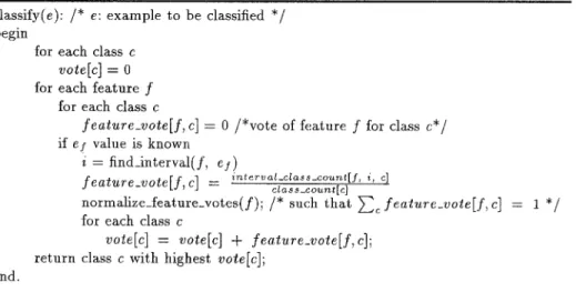
the interval on feature dimension f into which e/ falls is searched, where e/ is the f value of the test example e. If e/ is unknown (missing), that feature gives a vote zero for each class. Hence, the features containing missing values are simply ignored. Ignoring the feature about which nothing is known is a natural a n d plausible approach.If
e]
is known, the interval i into which ef falls is found. For each class c, feature f gives a vote equal tofeature_vote[f, c] = interval_class_count[f, i, c]
class_count[c]
where
interval_class_count[f, i, c]
is the number of examples of class c which f a l l into interval i of feature dimension f . If e / f a l l s on the boundary of two intervals i and i + 1 of a linear feature, then a vote equal to the average of the votes suggested by the intervals i and i + 1 is given. For nominal features, only point intervals are constructed and each value must fall in an interval. The individual vote of feature f for classc, feature_vote[f, c],
is then normalized to have the sum of votes of feature f equal to 1. Hence, the vote of feature f is a real-valued vote less than or equal to 1. Each feature f collects its votes in an individual vote vector <vote/,1,..., votef,k
>, wherevote],c
is the individual vote of feature fclassify(e): /* e: example to be classified */ begin
for each class c vote[c] = o for each feature f
for each class c
f e a t u r e _ v o t e [ f , c] = 0 /*vote of feature f for class c*/ if e 4, value is known
i = find_interval(f, el)
f eature_vote[f , c] = i,~t .. . . l_c~ .. . . tU, i, ~] class-count[c]
normMize_feature_votes(f); /* such that ~ c f e a t u r e _ v o t e [ f , c] = 1 */ for each class c
vote[c] = vote[c] + feature_vote[f,e]; return class c with highest vote[c];
end.
Fig. 2. Classification in the VFI Algorithm.
for class c and k is the n u m b e r of classes. Then the individual vote vectors are s u m m e d up to get a total vote vector < v o t e 1 , . . . , votek >. Finally, the class with the highest total vote is predicted to be the class of the test instance.
A class is predicted for the test instance in order to be able to measure the p e r f o r m a n c e by percentage of correct classifications on unseen instances in the experiments. With this implementation, V F I is a categorical classifier, since it
~otqq
returns a unique class for a test instance [6]. Instead, ~ k ~otqk] can be used as the probability of class c which makes V F I a more general classifier. In t h a t case, V F I returns a probability distribution over all classes.
2.2 A n E x a m p l e
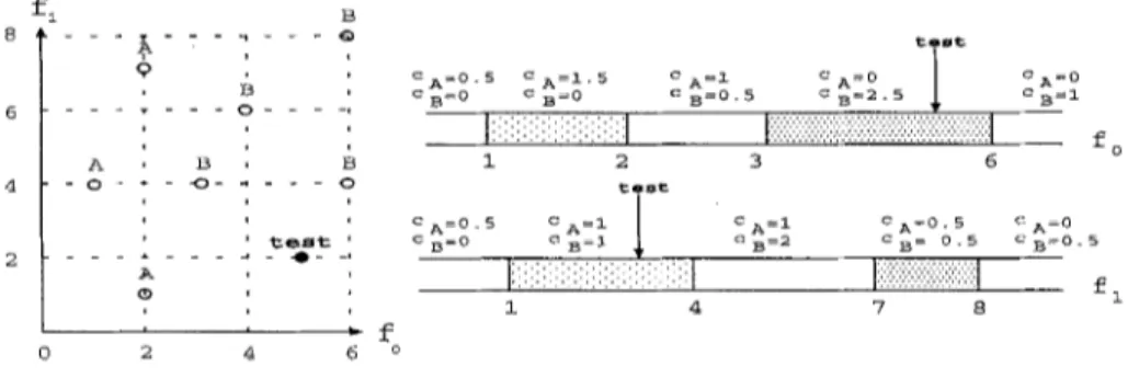
In order to describe the V F I algorithm, consider the sample training dataset on the left of Figure 3. In this dataset, we have two linear features f0 and f l , and there are 3 examples of class A and 4 examples of class B. T h e constructed concept description after the training phase is shown in Figure 3. There are 5 intervals for each feature. T h e lower bound of the leftmost intervals is - I N F I N I T E and the upper bound of the rightmost intervals is I N F I N I T E . T h e second interval on feature dimension of f0 can be represented as < 1, 1.5, 0 >, where 1 is the lower bound of the interval, 1.5 is count of training instances of class A, and 0 is the count of training instances of class B t h a t falls into t h a t interval.
In order to describe the classification phase of the V F I algorithm, consider a test example test = < 5, 3, ? >. On feature f0 dimension , the testo = 5 falls into the fourth interval as shown with an arrow in Figure 3. T h a t interval has
f~ B Q 6 - - - O . . . . , A B B 4 - O - + - ~ - ~ - - - O ' t ~ S t ' A O . f 2 4 6 ~
oi -t
C A = 0 . 5 C A = I . 5 C A = l C A = 0 C A = 0 c B = 0 c B = 0 c B = 0 , 5 c B = 2 . 5 c B = I I iiiiiii!i!i!i!iii!!!i I liiiii[iiii!i!iiiii[iiiii!iii!i[iii!i!i!iiiiiiiiiiiii!i[iiiiiiiiiiiiiii] f 0 1 2 3 6 t i s t c A = 0 5 c A = I c A = I c A = 0 . 5 c A = 0 c B = 0 C B = l C B = 2 C B = 0 . 5 c B = O - 5l!i!i!!iii!i!i!i!i!ii!!!!
iiiil
l!i!!ii!iiiiiiiiiii!iiiiiiiiiii!J
f
l 4 7 8
Fig. 3. A sample training dataset and the concept description learned by VFI.
a count c A = 0 for class A and a count C B : 2.5 for class B, so the vote vector of f0 is voteo =< 0/3, 2.5/4 >. The normalized vote vector is voteo =< O, 1 >. This means that feature f0 votes 0 for class A and 1 for class B. On the other feature dimension, test example falls into the second interval. T h a t interval has a count CA = 1 for class A and a count cB = 1 for class B, so the vote vector of fl is vote1 = < 1/3, 1/4 >. The normalized vote vector is vote1 = < 0.57, 0.43 >. Finally, the votes of the two features are s u m m e d up correspondingly and total vote vector is vote = < 0.57, 1.43 >. VFI votes 0.57 for class A and 1.43 for class B, so class B with the highest vote is predicted as the class of the test example.
3 E v a l u a t i o n o f t h e V F I A l g o r i t h m
This section presents the space and time complexity analyses and the empirical evaluation of VFI. The VFI algorithm is compared with CFP, k-NNFP, and NBC in terms of classification accuracy, and training and testing times.
3.1 C o m p l e x i t y A n a l y s i s
The VFI algorithm represents a concept description by feature intervals on each feature dimension. Each feature dimension has at most 2k + 1 intervals where k is the number of classes. Each interval requires k + 1 m e m o r y units, one for the lower bound of the interval and k for the count of each class. So each feature dimension requires (2k + 1)(k + 1) space and since there are d features, the total space requirement of the VFI algorithm is d(2k + 1)@ + 1) which is O(dk2). On the other hand, the space requirement of NBC is O(m) at worst case, where m is the number of training instances.
In the training phase of the VFI algorithm, for each training instance the corresponding intervals on each feature dimension is searched and the counts of corresponding classes are incremented. Since there are m training instances, d feature dimensions, and at most 2k + 1 intervals on each feature dimension, this makes up md(2k + 1) total, which is O(mdk). Hence, the training time of VFI increases with the number of features and classes, and the size of the dataset.
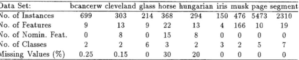
Table 1. Properties of the real-world datasets used in the comparisons. Data Set:
No. of Instances No. of Features No. of Nomin. Feat. No. of Classes Missing Values (%)
bcancerw cleveland glass horse hungarian iris musk page segment
699 303 214 368 294 150 476 5473 2310
9 13 9 22 13 4 166 10 19
0 8 0 15 8 0 0 0 0
2 2 6 3 2 3 2 5 7
0.25 0.15 0 30 20 0 0 0 0
On the other hand, the training time complexity of NBC is
O(vdm),
where v is the average number of distinct values per feature. Hence, the training time of NBC increases with the number of features and distinct values per feature, and the size of the dataset. Since in real-world datasets k < < v especially for linear features, the training time for VFI is less than that of NBC.In the classification phase of the VFI algorithm, for each feature, the interval that the corresponding feature value of the test example falls into, is searched and the individual votes of each feature is summed up to get the total votes. Since there are at most 2k + 1 intervals on each feature dimension and there are d features, the classification phase takes at worst case d(2k + 1) which is
O(dk).
Hence, the testing time of VFI increases with the number of features and classes. The test time complexity of NBC isO(dkv),
which means that the testing time of NBC increases with the number of features, distinct values per feature, and classes. Since an extra factor of v does not exist in the complexity of VFI and in real-world datasets k < < v especially for linear features, the testing time for VFI is less than that of NBC.3.2 E m p i r i c a l E v a l u a t i o n o n R e a l - W o r l d D a t a s e t s
In this section we present an empirical evaluation of the VFI algorithm on real- world datasets provided by the machine learning group at the University of California at Irvine [7]. An overview of the datasets is shown in Table 1. The features V3, V25, V26, V27, and V28 are deleted from the original Horse-colic (called horse in the tables) dataset and feature V24 is used as the class. The dataset Page-blocks is also called as page in short. The classification accuracy of the algorithms is used as one measure of performance. The most commonly used classification accuracy metric is the percentage of correctly classified instances over all test instances. 5-fold cross-validation technique, which ensures t h a t the training and test sets are disjoint, is used to measure the classification accuracy in the experiments. In addition to the accuracy comparisons, the average running time of the algorithms are also compared.
The classification accuracies of CFP, k-NNFP (k = 1), VFI, and NBC ob- tained by 5-fold cross-validation on nine real-world datasets are given in Table 2. VFI usually outperforms k-NNFP but sometimes C F P outperforms VFI where
Table 2. Classification accuracy (%) of VFI, NBC, CFP, and k-NNFP (k = 1) obtained by 5-fold cross-validation on nine real-world datasets.
Data Set: bcancerw cleveland glass horse hungarian iris musk page segment
X/FI 95.14 82.49 5 7 . 4 8 7 9 . 3 5 8 2 . 6 2 9 5 . 3 3 77.73 87.39 77.02
NBC 97.28 80.84 52.34 8 0 . 9 6 82.94 92.0 71.68 8 9 . 8 80.74
CFP 95.85 83.82 5 4 . 1 7 8 1 . 5 3 8 1 . 5 9 94.67 60.49 89.77 66.75
k-NNFP 94.0 67.62 57.0 66.84 70.04 90.0 69.54 90.52 75.1
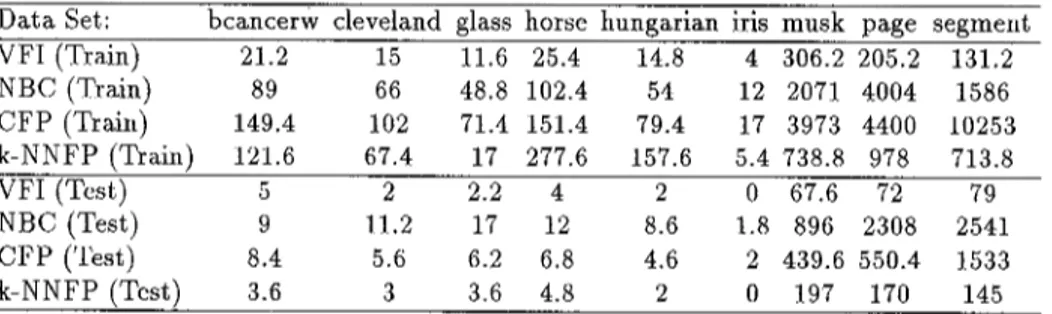
Table 3. Average running times (msec.) of VFI, NBC, CFP, and k-NNFP (k = 1) on a SUN/Sparc 20/61 workstation. Training is done with 4/5 and Testing with 1/5 of the dataset. 0 means time is less than 1 msec.
Data Set: V F I (Train) NBC (Train) c s p (Train) k-NNFP (Train) VFI (Test) NBC (Test) CFP (Test) k-NNFP (Test)
bcancerw cleveland musk page segment
21.2 15 11.6 25.4 14.8 4 306.2 205.2 131.2 89 66 48.8 102.4 54 12 2071 4004 1586 149.4 102 71.4 151.4 79.4 17 3973 4 4 0 0 10253 121.6 67.4 17 2 7 7 . 6 157.6 5.4 738.8 978 713.8 5 2 2.2 4 2 0 67.6 72 79 9 11.2 17 12 8.6 1.8 896 2 3 0 8 2541 8.4 5.6 6.2 6.8 4.6 2 439.6 550.4 1533 3.6 3 3.6 4.8 2 0 197 170 145
glass horse hungarian iris
C P P is given some parameters. In four of the datasets V F I outperforms NBC, in other four NBC performs better, and in Hungarian dataset they perform equally. The largest differences in accuracy are observed on the Glass and the Musk datasets on which VFI outperforms NBC.
The superiority of V F I over NBC is indeed in its speed. The average training and testing run times of all classifiers are given in Table 3. It is observed that V F I is always faster than NBC both in training and testing as expected due to the reasons discussed in Section 3.1. VFI is in fact the fastest classifier a m o n g four classifiers in terms of both training time and testing time on all datasets with the only exception of the Bcancerw dataset where k - N N F P is slightly faster only in testing. Table 3 also shows that both train and test time of all the classifiers on large datasets like Page-blocks and Segment are larger than that of smaller datasets. The larger run times of all classifiers on the Musk dataset than that of smaller ones shows the effect of the number of features on the run times.
4 C o n c l u s i o n s
The VFI classifier has similarities with the Naive Bayesian Classifier, in that they both consider each feature separately. Since each feature is processed separately,
the missing feature values that may appear both in the training and test instances are simply ignored both in NBC and VFI. In other classification algorithms, such as decision tree inductive learning algorithms, the missing values cause problems [9]. This problem has been overcome by simply omitting the feature with the missing value in both NBC and VFI. Another advantage of both classifiers is that they can make a general classification returning a probability distribution over all classes instead of a categorical classification [6]. Also note that the VFI algorithm, in particular, is applicable to concepts where each feature can be used in the classification of the concept independently. One might think that this requirement may limit the applicability of the VFI, since in some domains the features might be dependent on each other. Holte has pointed out that the most datasets in the UCI repository are such that, for classification, their features can be considered independently of each other [4]. Also Kononenko claimed that in the data used by human experts there are no strong dependencies between features because features are properly defined [5].
The e• results show that VFI performs comparably and even bet- ter than NBC and usually better than C F P and k - N N F P on real-world datasets. Moreover, VFI has a speed advantage over CFP, k-NNFP, as well as NBC, which is known to be a fast classifier.
For future work, we plan to integrate a feature weight learning algorithm to VFI, since both relevant and irrelevant features have equal voting power in this Version of VFI. Genetic algorithms can be used to learn weights for VFI [2] as well as several other weight learning methods [101.
R e f e r e n c e s
1. Akku~, A., & Gfivenir, H. A. (1995). K Nearest Neighbor Classification on Feature Projections. Proceedings of ICML '96, 12-19.
2. DemirSz, G., &: Giivenir, H. A. (1996). Genetic Algorithms to Learn Feature Weights for the Nearest Neighbor Algorithm. Proceedings of BENELEARN-96, 117-126. 3. Giivenir, H. A., & ~irin, I. (1996). Classification by Feature Partitioning. Machine
Learning, Vol. 23, 47-67.
4. Holte, R. C. (1993). Very simple classification rules perform well on most commonly used datasets. Machine Learning, Vol. 11, 63-91.
5. Kononenko, I. (1993). Inductive and Bayesian Learning in Medical Diagnosis. Ap- plied Artificial Intelligence, Vol. 77 317-337.
6. Kononenko, I. & Bratko, I. (1991). Information-Based Evaluation Criterion for Clas- sifier's Performance. Machine Learning, Vol. 6, 67-80.
7. Murphy, P. (1995). UCI Repository of machine learning databases, [Anonymous FTP from ics.uci.ed~ in the directory pub/macMae-learning data.base@ Department of Information and Computer Science, University of California, Irvine.
8. Quinlan, J. R. (1986). Induction of decision trees. Machine Learning, Vol.1, 81-106. 9. Quinlan, J. R. (1989). Unknown attribute values in induction. Proceedings of 6th
International Workshop on Machine Learning, 164-168.
10. Wettschereck,D. & Aha, D. W. (1995). Weighting Features. Proceedings of the First International Conference on Case-Based Reasoning (ICCBR-95).