THE REPUBLIC OF TURKEY
BAHÇESEHIR UNIVERSITY
LEAD TIME REDUCTION: MACHINE INTERFERENCE
PROBLEM IMPACT ON
LEAD TIME
Master ThesisAHMED ELSHERIF
THE REPUBLIC OF TURKEY
BAHÇESEHIR UNIVERSITY
LEAD TIME REDUCTION: MACHINE
INTERFERENCE PROBLEM IMPACT ON
LEAD TIME
Master ThesisAHMED ELSHERIF
Supervisor: ASSIST. PROF. Dr. BAŞAK AKDEMİR
T.C.
BAHÇESEHIR UNIVERSITY
THE GRADUATE SCHOOL OF NATURAL AND APPLIED SCIENCES INDUSTRIAL ENGINEERING
Title of the Master’s Thesis : LEAD TIME REDUCTION: MACHINE
INTERFERENCE PROBLEM IMPACT ON LEAD TIME Name/Last Name of the Student : Ahmed ELSHERIF
Date of Thesis Defense : 28.05.2018
The thesis has been approved by the Graduate School of the Graduate School of Natural and Applied Sciences.
Assist. Prof. Yücel Batu SALMAN Graduate School Director
Signature
I certify that this thesis meets all the requirements as a thesis for the degree of Master of Science.
Assist. Prof. Dr. Adnan ÇORUM Program Coordinator
Signature
This is to certify that we have read this thesis and we find it fully adequate in scope, quality and content, as a thesis for the degree of Master of Science.
Examining Committee Members Signature
Thesis Supervisor
Assist. Prof. Dr. Başak AKDEMIR ---
Member
Prof. Dr. F. Tunç BOZBURA ---
Member
Prof. Dr. Selim ZAIM ---
ACKNOWLEDGEMENT
I would like to extend my sincere gratitude to my advisor Assist. Prof. Dr. Başak Akdemir for her constant guidance, endless help, patience, knowledge, and precious support throughout this thesis.
My deepest gratitude goes to general manager, supervisors, team leader, operators and everyone who stood by me throughout this thesis from SML TR family.
I would like to express my gratitude to all my friends and family for their endless encouragement, my parents for giving me their endless support and passion.
Lastly, I would like to express my gratitude to everyone who supports and believe in me.
IV ABSTRACT
LEAD TIME REDUCTION: MACHINE INTERFERENCE PROBLEM IMPACT ON LEAD TIME
Ahmed Elsherif
Industrial Engineering
Thesis Supervisor: Assist. Prof. Başak AKDEMİR
May 2018, 43 pages
Customer satisfaction is one of the most important keys for surviving in a high competition markets. Short lead time expectation by customers drives managers of production systems to be eager to continually improve and develop their systems. The following work of thesis considers an appropriate method for lead time reduction in many industrials where one operator operates several machines. Machine interference problem (MIP) has a significant role in those production systems. Therefore, a revised method for allocating the optimum number of similar machines to operators, developed by Hadad and Keren had been used to find the optimum number of machines should be assigned for each operator to improve MIP; Two objective used to get the optimum number of machines per operator maximizing profit and minimizing cost. A quantitative analysis of average service time and run time had been calculated to get the most accurate results before applying them in the revised allocating model. This method used to increase the machine utilization, decrease average cycle time and increase productivity to decrease lead time and increase customer satisfaction.
A real case study illustrates the applicability of the proposed method for lead time reduction. The final finding shows increases of machine utilization, productivity which reduce lead time and increase customer satisfaction.
V ÖZET
ÜRETIM SÜRESINDE TASARRUF: MAKINA GIRIŞIM PROBLEMININ ÜRETIM SÜRESI ÜZERINDEKI ETKISI
Ahmed Elsherif
Endüstri Mühendisligi Yüksek Lisans Programi
Tez Danismani: Dr. Öğr. Üyesi Başak AKDEMİR
Mayıs 2018, 43 sayfa
Müşteri memnuniyeti, yüksek rekabet pazarlarında hayatta kalmak için en önemli anahtarlardan biridir. Müşteriler tarafından kısa teslim süresi beklentisi, sistemlerini sürekli iyileştirme ve geliştirmeye istekli olmak için üretim sistemlerinin yöneticilerini yönlendirir. Aşağıdaki tez çalışması, bir operatörün birkaç makineyi çalıştırdığı birçok endüstride kurşun zamanı azaltımı için uygun bir yöntem olduğunu düşünmektedir. Makine Girişim Problemi (MIP), bu üretim sistemlerinde önemli bir role sahiptir. Bu nedenle, Hadad ve Keren tarafından geliştirilen operatörler için en uygun sayıda benzer makinenin tahsis edilmesine yönelik revize edilmiş bir yöntem, MIP'yi iyileştirmek için her operatör için optimum sayıda makinenin atanması için kullanılmıştır; İki hedef, operatör başına karı maksimize eden ve maliyeti en aza indiren optimum makine sayısını elde etmek için kullanılır. Bu nedenle, Hadad ve Keren tarafından geliştirilen operatörler için en uygun sayıda benzer makinenin tahsis edilmesine yönelik revize edilmiş bir yöntem, MIP'yi iyileştirmek için her operatör için optimum sayıda makinenin atanması için kullanılmıştır; İki hedef, operatör başına karı maksimize eden ve maliyeti en aza indiren optimum makine sayısını elde etmek için kullanılır. Revize edilen tahsisat modeline uygulanmadan önce en doğru sonuçların elde edilmesi için ortalama servis süresinin ve çalışma süresinin niceliksel bir analizi hesaplanmıştır. Bu yöntem, makine kullanımını arttırmak, ortalama döngü süresini ve tedarik süresini kısaltmak ve müşteri memnuniyetini arttırmak için üretkenliği arttırmak amacıyla kullanılmıştır.
Gerçek bir vaka çalışması, önerilen yöntemin kurşun zamanı azaltımı için uygulanabilirliğini göstermektedir. Son bulgular, makine kullanımının, kurşun süresini azaltan ve müşteri memnuniyetini artıran üretkenliği arttırmaktadır.
VI CONTENTS TABLES VIII FIGURES IX ABBREVIATIONS X SYMBOLS XI 1. INTRODUCTION 1 2. LITERATURE REVIEW 3
2.1 LEAD TIME IDENTIFICATION 3
2.1.1 Lead time significant factors and variability 3
2.1.2 Lead time improvement investment 5
2.1.3 Lead time classification 6
2.2 PRODUCTIVITY 6
2.3 MACHINE EFFICIENCY 7
2.3.1 Production breakdown 8
2.3.2 Machine efficiency measurements 8
2.3.2.1 Availability 9
2.3.2.2 Performance 9
2.3.2.3 Quality 9
2.3.2.4 Overall Equipment Effectiveness 10
2.4 OPERATORS AND MANPOWER UTILIZATION 10
2.4.1 Measuring Manpower utilization 10
2.5 MACHINE INTERFERENCE PROBLEM 11
2.5.1 The revised method for allocating optimum number of similar Machines to operator calculations 14
3. METHODOLOGY 17
4. APPLICATION OF PRODUCTION LEAD TIME IMPROVEMENT 20
4.1 PROBLEM DEFINITION 21
4.2 OVERALL EQUIPMENT EFFECTIVENESS ANALYSIS 23
VII
4.3.1 Run Time Analysis 25
4.3.2 Service Time Analysis 26
4.3.2.1 Setup Time Study 26
4.3.2.2 Packaging Time Study 27
4.3.2.3 Minor Stops Time Study 28
4.3.2.4 Change Rollers Time Study 28
4.3.3 Revised method for allocating the optimum number of similar Machines to operators Application 29
4.3.3.1 Optimal number of machines to operators 29
4.3.3.2 Optimal number of operators 32
4.4 IMPROVEMENT OF THE PROPOSED SOLUTIONS 34
5. DISCUSSION AND RECOMMENDATION 35
6. CONCLUSION 37
REFERENCES 38
APPENDICES
Appendix A.1 Interference Rate according to the Revised method for allocating the optimum number of similar machines to operators 45 Appendix A.2 Collected Data for OEE and Manpower utilization
measurements 46
Appendix A.3 Cutting Machines Models and Method of Cutting Methods 47 Appendix A.4 Run time collected data and Regression models 48 Appendix A.5 Weighted average length data and calculation 62 Appendix A.6 Setup time collected data and calculations 99 Appendix A.7 Packaging time collected data and calculations 104 Appendix A.8 Minor stops time collected data and calculations 106 Appendix A.9 Change rollers time collected data and calculations 108 Appendix A.10 Machine utilization and work load Time Series plots 110
VIII TABLES
Table 4.1: 2016-2017 monthly sales……… 22
Table 4.2: OEE and manpower analysis results 23
Table 4.3: Orders classification and quantity percentage 27
Table 4.4: Number of packets needed per unit 27
Table 4.5: Run time and service time ratio 29
Table 4.6: Financial data 29
Table 4.7: TCU and hourly profit 30
Table 4.8: Total hourly profit First Alternative 32 Table 4.9: Total hourly profitSecond Alternative 32 Table 4.10: Total hourly costFirst Alternative 33 Table 4.11: Total hourly costSecond Alternative 33 Table 4.12: Monthly production of the proposed solution 34 Table 4.13: Increase rate of the proposed solution 34 Table 5.1: Proposed improvement methods increase rates evaluation 35
IX FIGURES
Figure 2.1: Significant Factors on Production Lines 7 Figure 2.2: General Breakdown of a Production Shifts 8
Figure 4.1: 2016-2017 Monthly Sales 22
Figure 4.2: OEE Histogram 24
Figure 4.3: Manpower utilization Histogram 24
Figure 4.4: Service Time Factors 26
Figure 4.5: Hourly Profit per Machine for one operator and N machines 31
X
ABBREVIATIONS
AM : Autonomous Maintenance ERP : Enterprise Resources Planning JIT : Just In Time
MIP : Machine Interference Problem MRP : Material Resources Planning OEE : Overall Equipment Efficiency PFL : Printing Fabric Labels Department SPC : Statistical Process Control
TL : Turkish Lira
XI SYMBOLS
Adjusted Cycle Time : HN
Average Hourly Profit :
N
Average Material Cost per unit : V
Average Run Time per unit for one machine : T
Average selling Price per unit : L
Average service Time per unit for one machine : t
Hourly Fixed Cost of one machine : CM1
Hourly Operator Cost : C
Hourly Variable Cost of one machine : CM2
Interference Time : tmi Interference Rate : Pt
N
MI
, Machine Utilization :
,N
N
Number of Machines : NNumber of machines need service : X
Operator Work Load : B
N
N
, Optimum number of machines to be assigned to each operator : N* Optimum number of operator for all machines : K*Probability of idle operator : P (x = 0)
Service Time to Run Time Ratio :
Total Cost per unit for N machines : TCUN
Total number of machines : M
1. INTRODUCTION
Managers of production systems are eager to maximize profit, reduce cost and achieve customer satisfaction with high market competition and short lead time expectation by customers. One of the key methods to accomplish those aims is to increase productivity. Improve machine interference problem is the key to increase productivity in many industrials where one operator runs several machines.
Finding the optimum number of machines to be assigned to one operator is the key to improve the machine interference problem (MIP). Improving MIP reduce the average cycle time which increase the productivity of the production system. On the other hand, improving MIP reduces lead time, help management to calculate lead time more accurate for customers and achieve customer satisfaction.
A common assumption in many interference models is that all machines are totally identical. However, in reality age, wear, and maintenance quality cause even those machines from the same manufacturer and the same type to be no longer identical. Hence, using of those models is insufficient before doing a time study for each machine to find the appropriate and accurate method to calculate average service time and run time to use in those models.
The point considered in this thesis is determining accurate number of machines to be assigned to one operator using a revised method for allocating the optimum number of similar machines to operators. Hence, decrease the average cycle time, increase productivity, reduce lead time and increase customer satisfaction. This method was applied for the two objectives increase profit and decrease cost. However, in real life firms have product variety, machines efficiency variety and lack of historical data for all the production processes; in this thesis, an average service time and run time calculated according to the available historical data and time study to apply them in the MIP models to get the most accurate results.
2
Chapter one is dedicated to presentation of the necessity of machine interference rate and problems of allocating the optimum number of machines to operators to increase productivity and lead time reduction.
Chapter two includes literature review of the published articles and previous works about lead time, productivity, machine interference problem MIP. After a general knowledge about lead time and productivity the calculations of overall equipment efficiency OEE methods are presented. Moreover, formulations of revised method for allocating the optimum number of similar machines to operators are given. Lastly, relation between MIP, productivity and lead time is told.
Chapter three is about methodology of thesis. Necessity and reason of proposed method discusses the data collection process and limitations in the collection and the aim of the thesis are included.
Chapter four includes application of proposed method. Firstly, a general knowledge is given about the firm where the proposed method is applied. The firm problem definition and necessity of proposed method is told. Then, application of methodology is exemplified by the real collected data. Lastly, the earnings of the proposed method are presented at the end of this chapter.
Chapter five provides a summary of the results of the study, recommendation and suggestions for future improvements for the firm.
3
2. LITERATURE REVIEW
Managers are eager to maximize profits and reduce cost of production to accomplish this target there are many important factors should be consider, monitor and improve (Tirkel and Rabinowitz, 2014). Customer satisfaction and lead time reduction should be improve in maximizing profit strategies (Kristoffersen, 2015). Moreover, increasing productivity one of the most important keys to increase profit and decrease costs (Bebeşelea, 2015). Otherwise, Hadad and Keren (2016) stated that one of the key methods used to accomplish those aims is to find the optimum number of operators needed to run the production lines. This thesis proposes a new vision to improve lead time and customer satisfaction by help managers to determine the optimal number of operators should be assigned to a given number of machines, and the number of machines should be run by each operator which increase the productivity and accomplish the manager’s target of minimizing production costs or maximizing profits.
2.1 LEAD TIME IDENTIFICATION:
There are many researchers studied lead time and all its relevant significant factors. In a make-to-order situation, lead time terms to the delay between the time of the customer’s demand and the time when the demand is completely satisfied while in a make-to-stock situation lead time terms to procurement lead time for obtaining materials from suppliers (Hill and Khosla, 1992). Lead time should be at the minimum level; therefore, analyzing lead time and its perspective are necessary in lead time reduction process (Kristoffersen, 2015).
2.1.1 Lead Time Significant Factors and Variability:
Supply chain management, inventory management, logistics, capital investing, MRP system, production capacity, production control, productivity, procurement, process robustness, process flow, work analysis, machines layout, machines efficiency, worker performance, outsourcing, and complementary products are the most common factors between all lead time reduction studies. Bottani and Rizzi (2008), De Toni and Meneghetti
4
(2000) defined lead time reduction process as a timing competition. Manufacturing strategy, operational management and production process management has a significant role on lead time reduction factors such as increase productivity, reduce unit cost, improve quality, decrease carrying cost, reduce the safety stock and decrease forecast horizon (Albey and Uzsoy, 2015; Chen and Wang, 2009; Hill and Khosla, 1992). Moreover, logistics, cost, inventory and service level to customer had been defined as significant factors to improve lead time by Cannella et al. (2017). In addition, reduce setup time, raw materials availability, reduce queue time, improving tools equipment and layouts had been defined as significant key factors to improve lead time by (Shirai and Amano, 2017; Hill and Khosla, 1992). Moreover, Shirai and Amano (2017) used the theory of constraints (TOC) which focused on the importance of how to avoid the bottlenecks in production processes. On the other hand, Cannella et al. (2017) defined limiting lead time variability by lean manufacturing, six sigma, improving outsourcing and integration as an effective factor in lead time reduction process.
Just in time (JIT) is one of the most effective key method of lead time reduction by improving the optimum way of production and inventory management (Ouyang et al. 2007; De Treville et al. 2004).
Supply Chain Management and all the internal and external logistics processes should be well managed to control lead time (Bottani and Rizzi, 2008). Moreover, De Treville et al. (2004) observed that the companies should give the first priority to improve supply chain performance which reduces the lead time duration instead of improving the supply chain transfer information system. Managers should start improve supply lead time then improve demand information transfer to reduce transaction uncertainty to get better improvement results (De Treville et al., 2004).
In addition lead time became more critical factor at markets which has a very sensitive price and demand lead time (Zhao et al. 2012; Ray and Jewkes, 2004). Therefore, after the first research appeared by Boyaci and Ray (2003) about the relation between lead time and pricing; Chen et al. (2017) developed a new model to find the optimal lead time and pricing
5
decision and observed that to get a shorter lead time from risk averse suppliers delay penalty cost should be at a certain level which drive suppliers to avoid this penalty cost.
Kristoffersen (2015) studied two partner organizations in the same value chain and observed that without accurate and efficient enterprise resource planning (ERP) system the operators and mangers will not be able to deal with the lack of the lead time and take the right decisions in the right time to improve the lead time and find the appropriate strategy plan. Simultaneously, many researchers studied the relation between the lead time and inventory management and figured out several models to manage this relation (Sarkar and Mahapatra, 2017).
2.1.2 Lead Time Improvement Investment:
How to invest capital is one of the most important and critical managerial decisions. Therefore, many studies discussed the relation between investing capitals in lead time reduction and if it has a significant effect or not (Lin, 2016). After studying the investment strategies of firms in market which has a stochastic dynamic setting by Genc (2017) he observed that there are two main types of firms strategy classification first one has a significant lead time or depend on time to build strategy and the other one without lead time value.
Firms can reduce the safety stock cost, reduce losses in the out of stock, improve their customer satisfaction and go further in the market competition by reducing their lead time (Chen et al., 2017; Lin, 2016; Ouyang et al., 2007). Moreover, Lin (2016) studied the effectiveness of increasing the investment to reduce the variability of the lead time and observed that there are three main factors should be consider which is how to drive the firm to reach the optimal production, integrated inventory and logistic policy with the optimal investment strategy to deal with the realistic and stochastic of lead time. In addition, Hill and Khosla (1992) found that in long term strategies the cost of reducing lead times becomes nothing in compare with the benefit and profits that the firm will get from reducing the lead time.
6 2.1.3 Lead Time Classification:
There are different types of lead time such as assembly lead time, procurement lead time, production lead time and demand lead time (Chen and Wang, 2009). This thesis focuses on the production lead time. Schmenner (2001) studied “theory of swift, even flow” and observed that firms which emphasize on flow, speed and reducing the variability can improve their productivity better than those emphasize productivity directly which has a significant effect on lead time. According to the previous literature review about lead time and its significant factors it became clear that it is very complicated and very networking; if firms want to improve lead time they have to improve their supply chain management by contrast if they want to improve their supply chain management they have to improve their lead time under the umbrella of supply chain. In addition some studies figured out that lead time is being effected with the management strategy and firms have firstly to improve their management strategy to improve their lead time. By contrast, many researchers argued that firms should firstly improve their production planning and management to improve their lead time. Therefore, it becomes clear that it is like a game of prioritizing and each firm should take the right way and put the suitable prioritizing system to their situation.
2.2 PRODUCTIVITY:
Evolution of the work load of the system overtime has a significant effect on lead time in firms (Albey and Uzsoy, 2015; Pahl et al., 2007; Missbauer, 2002). Moreover, Azizi (2015) stated that improving production performance such as productivity, equipment, efficiency and process control became the most important key for firms to survive in the competitive market. Therefore many studies focused on this point (Chen and Wang, 2009). Otherwise, continuous improvement in production capability became necessary for firms to survive and to overcome all the uncertainty in the production performance indicators. Therefore Azizi (2015) studied the relation between the overall equipment effectiveness (OEE), statistical process control (SPC) and autonomous maintenance (AM) to evaluate production productivity by continuously improve process control and machine efficiency and observed that to improve quality, production productivity, reduces defects, reduce wastes and
7
customer satisfaction firms should use statistical process control (SPC). On the other, hand to measure the effectiveness of machines, availability, quality and performance rate firms should use overall equipment efficiency (OEE) (Azizi, 2015;Soković et al., 2009). While Wudhikarn (2011) defined the six big losses which affect the machine performance as setup and adjustments, reduced speed, periodic small stops or minor stops, start up rejects and defected and rejected products. Therefore; Azizi (2015) applied statistical process control (SPC) and overall equipment efficiency (OEE) in a tiles manufacturing company and observed that increase productivity had been affected by minimizing the defect rate and maximizing the machine performance.
2.3 Machine Efficiency:
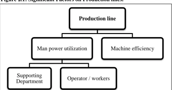
Production managers should accurately interpret all the relevant production data to identify the significant factors at the production line and to immediately take the right decisions to improve productivity, utilization of resources, manpower utilization, machine efficiency and the all over efficiency (Subramaniam et al. 2008). Significant factors on production lines were classified by Subramaniam et al. (2008) into three main levels as shown below in figure 2.1.
Figure 2.1: Significant Factors on Production lines.
Source: Subramaniam et al. (2008)
Production line
Man power utilization
Supporting
Department Operator / workers
8 2.3.1 Production Breakdown
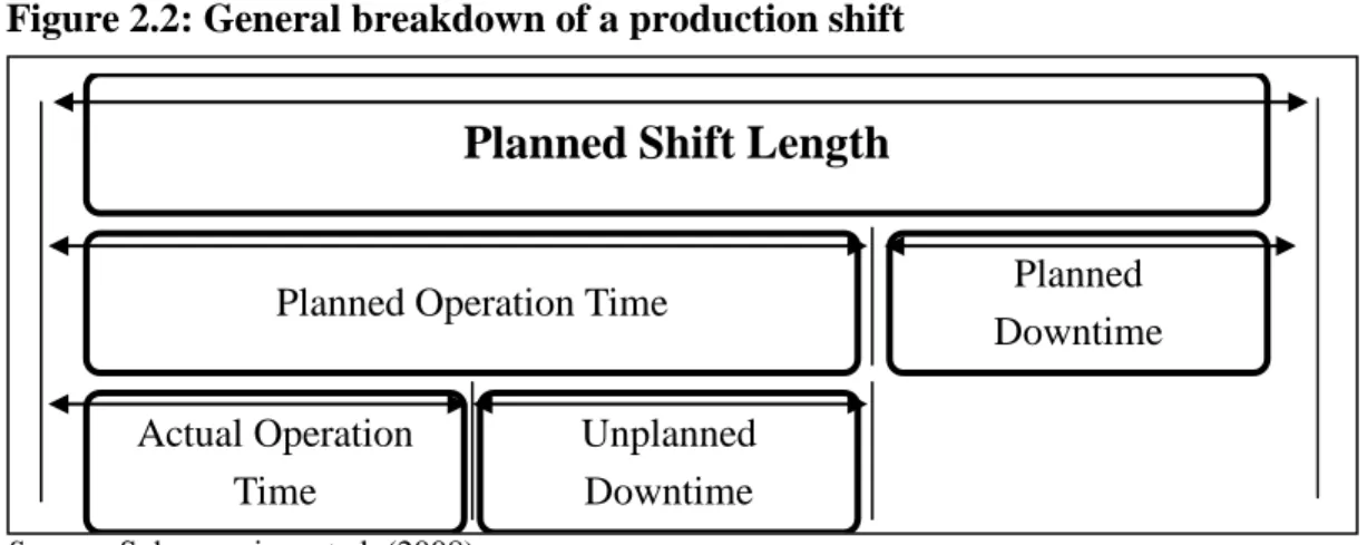
Planned operation time is classified into two major factors which is actual operation time and unplanned downtime. Hence, identifying planned operation time measurements is the key to help managers to measure machine efficiency and manpower utilization (Subramaniam et al. 2008). Therefore, to improve the production capacity managers are eager to maximize the actual operation time as much as possible and minimize the unplanned downtime to achieve their target (Wudhikarn, R., 2011). Production planning time can be classified as shown in figure (2.2).
Figure 2.2: General breakdown of a production shift
Source: Subramaniam et al. (2008)
2.3.2 Machine Efficiency Measurements
Optimization of machineries in higher rate of production output industry is a common target between all managers to get the maximum usage of machineries in the shortest time possible. Manufacturing productivity losses had been classified into three main factors Availability, Performance and Quality under the Overall Equipment Effectiveness (OEE) umbrella to monitoring and improve the manufacturing efficiency. Measuring those factors used as a gauge to measure efficiency and improve productivity (Wudhikarn, 2011; Subramaniam et al. 2008). Planned downtime such as (meal breaks, scheduled maintenance and planned stops of production) is excluded from the overall time losses such as unplanned failure, breakdowns, material shortage and changeover time to get the actual operation time.
Planned Shift Length
Planned Operation Time
Actual Operation Time Unplanned Downtime Planned Downtime
9 2.3.2.1 Availability
All events which can stop the production process such as material shortage, equipment failures and changeover time are included while calculating the downtime loss to figure out the availability. The changeover time should be included in OEE analysis when it is not be possible to eliminate and became a part of downtime. Actual operation time is the remaining available time. Therefore, availability simply calculated as the ratio of operation time to planned operation time. Availability is calculated according to equation 2.1 (Subramaniam et al. 2008; Sheu, 2006).
Time Operation Planned Time Operation Actual ty Availabili (2.1) 2.3.2.2 Performance
Performance is affected by all factors which produce a speed loss in production cycle time which included operator inefficiency, substandard materials and machine. Actual operation time is the remaining available time. Therefore, the ratio of actual operation time to planned operating time calculated the performance. The minimum cycle time that the process could be done within under optimal conditions for a given product is defined as machine ideal cycle time. Hence, performance could be calculated according to equation 2.2 (Subramaniam et al., 2008; Sheu, 2006)
Time Operation Planned produced pices Total Time Cycle Ideal Machine = e Performanc (2.2) 2.3.2.3 Quality
Quality loss is all the quality rejected products or products that require rework. Productive time is the remaining time. The production planning target is to maximize the actual productive time. Quality is the ratio of actual productive time to planned operation time. Quality could be calculated according to equation 2.3 (Subramaniam et al., 2008; Sheu, 2006). Produced Pieces Total Produced Pieces Good = Quality (2.3)
10 2.3.2.4 Overall Equipment Effectiveness
Overall equipment effectiveness (OEE) is a combination between Availability, performance and quality to become one score to provide a final measure of machine efficiency. The ratio of actual production time to planned production time is called OEE which could be calculated according to equation 2.4 (Subramaniam et al., 2008; Sheu, 2006)
Quality e Performanc ty Availabili OEE (2.4) 2.4 Operators and Manpower Utilization
Management objectives will not be able to accomplish in industrial production without improving the manpower utilization which classified into two factors first, the direct operators which are the operators on the production line and second, indirect operators which are the operators in the supporting department. Human performance is one of the most important indicators of the planned production time. In case of the operator performance decrease or drop, production output will be directly effect in the same way. By contrast, if the operator performance increase and improve attitude production output will be directly increased. Once the managements faced unmet target it became so important to measure the operators performance to eliminate the wasted time and increase productivity (Subramaniam et al., 2008).
2.4.1 Measuring Manpower Utilization
All the human factors that cause losses at speed base on the cycle time or time study in the production process are consider under manpower utilization measurement. Operator’s inefficiency is the major factor on measuring the performance of manpower utilization. Manpower utilization could be calculated according to equation 2.5.
output production Target output Production Actual = tilization Manpower U (2.5)
11 2.5 Machine Interference Problem (MIP)
In some cases and industrials such as textile, food, plastic, electronic, and rubber industries which have a multi machine assignment, it became difficult to calculate machine efficiency because of the machine interference problem (MIP). Machine Interference time is the waiting times for each machine which need service before the operator come to serve it. Machine Interference can be described as a system which consisting of number of machines and operators and each machine operates until it needs attention from the operator (Engin, 2010). At this kind of work stations system the number of machines is always greater than the number of operators. Machine interference problem appeared when one of those machines stop or required serving by an operator (Engin, 2010). In an industrial investigation, the machine interference time may be ten percent of machine time (Chien et al., 2014).
Hadad and Keren (2016) stated that allocating the optimum number of operators to run machines is the key to achieve the manager’s target which is increase the profit and decrease the cost. Several papers studied the machine interference problem from different point of views; Most of these paper are so old but recently the interest of MIP and its related topics has remained high (Ke and Wu, 2012). This multi machine system and machine interference problem should be considered while calculating and measuring the machine efficiency (Engin, 2010).
Hadad and Keren (2016) noted that Stecke and Aronson (1985) in their review about machine and operators models stated that there is a critical MIP decision related to have too few or too many machines to each operator. On the other hand, (Ilani et al., 2014) used in their paper to “reduction approach to the two-campus transport problem” the “partitioning problem with additive objective with an application to optimal inventory groupings for joint replenishment” method which was proposed by Chakravarty et al. (1982) to find the optimum of the partitions by transferring the problem to find the shortest path. Moreover, Yang et al., (2005) in their study about queuing network models with MIP stated that when
12
the system has a bottleneck and if the change of equipment and system is so expensive MIP became more critical and important.
Gupta (1997) considered the MIP with warm standby machines/tools in which the server takes a vacation of random duration and the repair facility becomes empty. They addressed the cases of multiple, single and hybrid multiple/single vacation schemes with exhaustive service. They provided a new transform free, closed form expressions for the probability distribution of the number of machines in the repair facility and the performance measures for MIP with warm standby machines/tools and server vacations. Ke and Wu (2012) studied the MIP between identical machines, repairmen and standby machines in an unreliable machines production system in their paper “Multi-server machine repair model with standbys and synchronous multiple vacation”. Moreover, Ke at el. (2013) used a modeled system as a finite-state Markov chain and obtained its steady state distribution by a recursive matrix approach considers a multi-repairmen problem comprising of number of operating machines with warm standbys machines subject to failures. They searched for the global optimal system parameters using the Quasi-Newton method and probabilistic global search Lausanne method. On the other hand, de Nitto Personè (2009) improved the machine interference model with vacation to deal with the recent problems of the communication area. Their model is extended to include parallelism in the vacation station and underlying Markov process is analyzed.
Kim and Lee (2012) studied the single server parallel machine scheduling problem, considering the setup for loading or unloading the product or handling tools on the machine using mixed integer programming formulations in their paper about “MIP models and hybrid algorithm for minimizing the makespan of parallel machines scheduling problem with a single server”
Chien et al. (2014) develop a methodology to determine the optimal assignment relationships between the test machines and the operators for different product mixes to improve utilization for the optimal system performance by using simulation, response
13
surface methodology, heuristic assignment and genetic algorithms to explore alternative assignment rations to identify well-performed assignment alternatives.
As noted by Hadad and Keren (2016) that several models used the binomial distribution for the MIP were surveyed by Stecke and Aronson (1985). Such as: Bernstein (1941), Weir (1944), Jones (1971), Gillespie and Wysowski (1974), Ackermann (1977) and Stecke and Solberg (1982). All these models assumed that a single operator is assigned to several machines. Moreover, Niebel and Freivalds (2003) gives an example for binomial interference calculations. On the other hand, Hadad et al. (2013) used multinomial distribution in their model of calculation the expected interference time in the queue for each service type. Gurevich et al. (2016) presented binomial and multinomial models for special cases of the MIP. While Hadad and Keren (2016) introduces a new method to determine the optimal number of operators needed to operate machines and calculate the interference rate accurately and simply by expected value calculations, without expressing the probabilities for each situation with machines down when the objective is maximizing the hourly profit/total cost unit.
Hadad and Keren (2016) proposed the first paper that proposes a method for calculation of the adjusted cycle time for the case where one operator runs a number of identical machines. Their study proposed a method for allocating the optimum number of identical machines to operators. Using the ratio between the service time and the run time, along with the number of machines assigned to one operator an interference tables that give the interference rate was included in their study. These tables can help determine the interference rates and the adjusted cycle time in order to compute the total cost per unit (TCU) and the hourly profit, the proposed method takes into account two types of cost: first, the hourly fixed cost of one machine. Second, the hourly operating cost of one machine and variable cost which is exists only when the machines are working, this cost is a function of the interference rate. The major differences between the common interference models are the assumptions related to the machine operating time distribution and the service time distribution. This model presented a simple method without any assumptions that relate to machine operating time distribution or service time distribution that enables
14
calculation of the interference rate using binomial distribution. By contrast, according to the common models calculation of the interference rate is complicated and needs the exact distributions of the operating time and the service time.
2.5.1 The revised method for allocating the optimum number of similar machines to operators’ calculations:
The value of PtM1
,N
is the interference rate is determined by
and the number of machines N as shown in Appendix A.1. The adjusted cycle time (H ) could be calculating N according the following procedure:a. Calculate the ratio between the service time and the run time using
t T.b. Calculate the interference rate PtM1
,N
by using the interference tables in Appendix A.1.c. Calculate the adjusted cycle time using equation (2.6) to, as follows:
N M M M N T t t H t H Pt N H H 1 1 1 1 1 ,
Pt
N
T N Pt H M M 1 , 1 , 1 1 1 1 (2.6)The yield per hour is
N N H N × 60 = Q units (2.7)
The machine utilization N was calculated according to following Equation (2.8):
The average utilization of machines, µN, is the ratio between the run time, T, and the
adjusted cycle time, HN The value of µ is calculated as shown in the following equation:
1 , 1 , 1 1 N , 1 1 N N Pt N Pt T T H T M M N (2.8)15
As much as the number of machines which is controlled by one operator, N increases, the interference ratePtM1
,N
increases, and the machine utilization,N decreases.The ratio between the total service time that the operator provides to the machinesNt and the adjusted cycle timeH is the average workload on the operatorN BN. The value of BN is calculated as follows in equation (2.9):
The probability that the operator is idle is equal to the probability that all the machines are running, that isP
X 0
. Therefore, the operator workload BN
,N
is the complementary event, specifically, that at least one machine needs service:
1 , 1 1 , 1 1 , Pt 1 N N Pt 1 N N B M N M N (2.9)As the number of machines that are run by one operator, N increases, the interference rate,
N
PtMI , increases, and the operator workload, BN
,N
also increases.TCUis the ratio between the total hourly cost (operator cost, machinery operating cost, and material cost) and the hourly yield obtained from N machines. The value of total hourly cost per unit TCU is calculated using equation (2.10) to produce HN N, which is given in
units of hours:
N N M N M N Q Q V C C C N TCU 1 2
CM
Pt
N
C V N C N Pt T TCU M M M N 1 2 1 1 , 1 1 , 1 1 (2.10)For a given number of M machines, one can calculate TCU for all the feasible values of N
M
N1 , , according to Equation (2.10) (note that for N = 1,PtMI
,N 1
0). The value of N that minimizes TCU will be denoted as N*. N* is the optimum number of N16
The average hourly profits per each machine
N when one operator runs N machines were calculated according to equation (2.11).
N Q TCU L N N N ) (2.11) However, in reality age, wear, and maintenance quality cause even those machines of the same type and from the same manufacturer to no longer be identical, a common assumption in many interference models is that all the machines are totally identical. In such cases the proposed method can be used by applying the average service ratio of all the machines. It is clear that a low variance of the service ratio among the machines increases the accuracy of the results. Chien et al. (2014) stated that improving MIP can increase the average cycle time. Therefore, in this thesis service time and run time analysis was used to increase the accuracy of results and to get more accurate service time and run time. “A revised method for allocating the optimum number of similar machines to operators” proposed by Hadad and Keren, (2016) used to allocate the optimum number of operators to run a number of machine, how many machines should be run by one operator. This thesis study the effect of the number of operators to avoid the MIP and increase productivity which is improves the Lead time.17
3. METHODOLOGY
Several lead time improvement methods have been developed for decades to meet different needs. Many books have been written and several journals are dedicated to improve lead time for different production systems and patterns. However, reduce lead time by improving machine interference problem (MIP) to increase productivity in many industrials where one operator runs several machines is a new developed method.
Finding the optimum number of machines to be assigned to one operator is the key to improve machine interference problem. Improving MIP reduce the average cycle time which increase the productivity of the production system. On the other hand, improving MIP reduces lead time, help management to calculate lead time more accurate for customers and achieve customer satisfaction.
A revised method for allocating the optimum number of similar machines to operators is the most recent model for MIP and the first method that proposes a method for calculation of the adjusted cycle time where one operator runs a given number of similar machines and a method for allocating the optimum number of similar machines to operators. According to the common models; the calculation of the interference rate is complicated and needs the exact distributions of operating time and service time. This model presents a method that enables calculation of the interference rate via binomial distribution, without any assumptions related to machine running time or service time distributions (Hadad and Keren, 2016).
This method could be done with the objective of maximizing profits, minimizing production costs, increasing productivity or setting a given load on the operators. Moreover, the method enables calculating various performance indexes such as workload, machine utilization and yield per hour. The deviation of this method from the observed hourly yield is 2.08 percent which is smaller than the deviations of all other tested models. This method can be applied even for cases where the machine running time and service time distribution functions are unknown. Furthermore, this method
18
needs as input only a single parameter the service ratio (the ratio between the service time and the run time). Hence, this method is applicable for any distributions of machine operating time and service time.
However, in reality age, maintenance quality, and wear cause even those machines from the same manufacturer and type to be no longer identical, a common assumption in many interference models is that all the machines are totally identical.Hence, using of those models is insufficient before doing a time study for each machine to find the appropriate and accurate method to calculate average service time and run time to use in those models.
However, in real life firms have product variety, machines efficiency variety and lack of historical data for all the production process; in this thesis, a quantitative analysis of average service time and run time used to calculate them according to the available historical data and time study to apply them in the revised allocating model to get the most accurate results.
Firstly, overall equipment effectiveness (OEE) and manpower utilization analysis had been used to analyze the machines efficiency and to figure out the significant factors which effect the production lead time from the six big losses (equipment failure, setup and adjustment, idling and minor stoppages, reduced speed of operation, process defects and reduced yield).
Secondly, the revised method for allocating the optimum number of similar machines to operators had been used to figure out the optimum number of operators needed for both objectives maximizing profit or minimizing cost. When viewed from this aspect, the normal average run time and service time method can be inaccurate according to the machines types and efficiency variability. Therefore, time study analysis had been done for each machine for both run time and service time to get the most accurate average time for them; after getting a regression model –using minitab- for each cutting machine for run time in terms of machine speed and product length using the maximum available speed and the weighted average length for a sample of 1619 different orders
19
and substituted in the regression equations to get the average run time for each cutting machine. Similarly, time study analysis had been done for service time which includes four main factors setup time, packaging time, products roll change time and minor stops time to get average service time for all cutting machines.
Finally, after analyzing the system and find out the optimum number of operators needed per shift; measuring increase of productivity, income and profit had been evaluated and suggest a standard method for production lead time calculation for each order to improve the lead time reduction and increase the customer satisfaction.
20
4. APPLICATION OF PRODUCTION LEAD TIME IMPROVEMENT
SML is a global business and branding solutions provider with 189 employees located in Beylikdüzü, Istanbul, Turkey. SML incorporating their innovative technologies with their partners -the world’s most prominent brands and retailers- to help them work smarter, higher quality and get long-term solutions. SML is presence in over 30 countries and based in Hong Kong.
SML TR was established in 2001 to satify the demands of the customers in a manner of total quality and best service in Turkey, Europe, Middle East and North Africa. SML is second in Turkish and the world’s Leadership and has a vision to lead the market by 2025. SML produce millions of tags, labels and tickets for the world’s leading retailers and brand owners every day utilizing various technologies such as online ordering E-Platform to help customers manage large amounts of complex data on a daily basis efficiently and accurately.
SML TURKEY Departments and Capacity:
i. Offset: working for two shifts with 18,000,000 – 25,000,000 pcs/month capacity using 60 percent of its capacity.
ii. Woven: working for two shifts with 10,000,000 – 12,000,000 pcs/month capacity using 60 percent of its capacity.
iii. Thermal Printing: working for one shift with 5,000,000 - 7,500,000 pcs/month capacıty using 60 percent of its capacity.
iv. PFL / Care Label: working for two shifts with 10,000,000 – 13,000,000 pcs/month capacıty using 55 percent of its capacity.
v. RFID: working for two shifts with 10,000,000 – 13,000,000 pcs/month capacıty using 50 percent of its capacity.
21
4.1 PROBLEM DEFINITION
Printing Fabric Labels (PFL) department has 6 printing machines and 13 cutting machines. Production process flow is printing, cutting, packaging, quality control and final packaging in sequence.
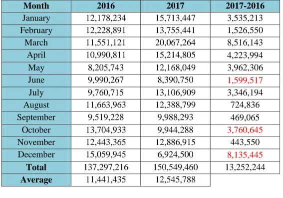
SML’s managers are eager to increase productivity to reduce products lead time to increase customer satisfaction which has a significant effect on the customer demand. Monthly sales quantity uncertainty between years 2016-2017 is shown in table 4.1 and figure 4.1. Cutting machines process has a bottle neck in the production process flow. PFL department works in two shifts, six days per week and has three operators assigned for all machines; maximum number of operating machines per shift only six to seven machines.
Overall equipment effectiveness (OEE) for all cutting machines had been discussed in section 4.2 and the Machine Interference Problem (MIP) had been discussed in section 4.3 and proposed an optimal solution for cutting machines to increase productivity and machine utilization by assigning the optimum number of machines to operator.
22 Table 4.1: 2016-2017 Monthly Sales.
Month 2016 2017 2017-2016 January 12,178,234 15,713,447 3,535,213 February 12,228,891 13,755,441 1,526,550 March 11,551,121 20,067,264 8,516,143 April 10,990,811 15,214,805 4,223,994 May 8,205,743 12,168,049 3,962,306 June 9,990,267 8,390,750 1,599,517 July 9,760,715 13,106,909 3,346,194 August 11,663,963 12,388,799 724,836 September 9,519,228 9,988,293 469,065 October 13,704,933 9,944,288 3,760,645 November 12,443,365 12,886,915 443,550 December 15,059,945 6,924,500 8,135,445 Total 137,297,216 150,549,460 13,252,244 Average 11,441,435 12,545,788
Figure 4.1: 2016-2017 Monthly Sales.
0 5,000,000 10,000,000 15,000,000 20,000,000 25,000,000 2016 2017
23
4.2 OVERALL EQUIPMENT EFFECTIVENESS ANALYSIS AND MAN
POWER UTILIZATION
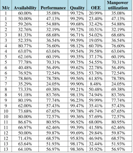
Table 4.2 shows the availability, performance, quality, OEE, and manpower utilization. Collected data will be presented in Appendix A.2. OEE calculated according to equation (2.4); Availability calculated according to equation (2.1); Performance calculated according to equation (2.2); Quality calculated according to equation (2.3) and manpower utilization calculated according to equation (2.5).
Table 4.2: OEE and Manpower Analysis Results
M/c Availability Performance Quality OEE
Manpower utilization 1 60.00% 35.08% 99.72% 20.99% 35.08% 1 50.00% 47.13% 99.29% 23.40% 47.13% 2 59.26% 54.88% 99.68% 32.42% 54.88% 2 32.76% 32.19% 99.72% 10.51% 32.19% 3 81.33% 68.68% 96.71% 54.02% 68.68% 3 52.35% 36.54% 99.59% 19.05% 36.54% 4 80.77% 76.60% 98.12% 60.70% 76.60% 4 63.07% 63.04% 99.54% 39.58% 63.04% 5 62.16% 60.19% 99.35% 37.17% 60.19% 5 77.78% 70.31% 99.75% 54.55% 70.31% 6 40.48% 56.49% 99.62% 22.78% 56.49% 6 76.92% 72.54% 96.35% 53.76% 72.54% 7 78.86% 78.78% 99.56% 61.85% 78.78% 7 35.29% 24.05% 99.90% 8.48% 24.05% 8 73.33% 69.38% 99.21% 50.48% 69.38% 8 91.18% 83.76% 98.13% 74.94% 83.76% 9 80.19% 77.74% 96.23% 59.99% 77.74% 9 62.00% 57.43% 99.47% 35.41% 57.43% 10 73.68% 67.65% 99.78% 49.74% 67.65% 10 80.00% 72.57% 99.36% 57.69% 72.57% 11 86.67% 80.95% 96.92% 68.00% 80.95% 11 66.97% 62.46% 99.39% 41.58% 62.46% 12 50.00% 59.87% 99.69% 29.84% 59.87% 12 71.43% 68.57% 95.83% 46.94% 68.57% 13 63.64% 51.93% 98.17% 32.44% 51.93% 13 64.10% 56.97% 98.36% 35.92% 56.97%
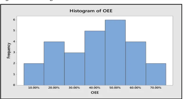
24 Figure 4.2: OEE histogram.
Figure 4.3: Manpower utilization histogram.
Figure 4.2 shows that twenty out of twenty six observations for OEE calculation for all machines are equal 50 percent or less and all observations are less than 70 percent. Moreover, figure 4.3 shows the uncertainty of manpower utilization calculations. Hence, Machine Interference Problem (MIP) had been discussed in section 4.3 to improve the OEE and manpower utilization to increase productivity and reduce production lead time.
70.00% 60.00% 50.00% 40.00% 30.00% 20.00% 10.00% 6 5 4 3 2 1 0 OEE Fr eq ue nc y Histogram of OEE 80.00% 70.00% 60.00% 50.00% 40.00% 30.00% 20.00% 7 6 5 4 3 2 1 0 Manpower utilization Fre qu en cy
25
4.3 THE MACHINE INTERFERENCE PROBLEM ANALYSIS
SML has thirteen cutting similar machines, three operators and two shifts. Revised method for allocating the optimum number of similar machines to operators has been applied to get the optimum number of machines to be assigned to each operator and to get the optimum number of operator to reduce interference rate, increase machine utilization and increase productivity. Two objectives have been proposed in this analysis to get the optimum solution; maximizing profit and decreasing costs.
Revised method for allocating the optimum number of similar machines to operators has a limitation – which was discussed clearly in literature review section- which is the assumption that all machines are totally identical. The ratio between run time and service time is necessary to use this method. Hence, a run time and service time analysis has been done as shown in section (4.3.1, 4.3.2) to get an accurate average run time and service time to produce one unit for all cutting machines to avoid method limitation.
4.3.1 Run Time Analysis:
SML has thirteen cutting machines with eleven different models as shown Appendix A.3. This variability required an analysis for each machine separately. Accordingly get an average run time for all machines. Machine speed level and products length are the two variable control machines run time; there are five machines do not have speed level indicator, therefore; an assumption that the maximum available speed was set for each product while taking the observations; hence, machine speed level is neglected in those five machines. Ten random observations for each machine had been taken to get a regression model for each machine in terms of product length and machine speed level for those machines which have machine speed level as will be presented in Appendix A.4. Maximum available speed and average products length had been used to get the average run time for each machine using regression models.
Hence, average products length was necessary; there were no direct available data for the average product length; therefore; 1,619 different printing order -14,633,965 pieces, collected from November 2017 and February 2018 historical data - used to get the average length. All wasted materials were neglected and weighted average method had been used to
26
avoid orders quantity effect on speed as will be presented in Appendix A.5; weighted average length is 111.79 mm and average run time is 6.81 min/unit.
4.3.2 Service Time Analysis:
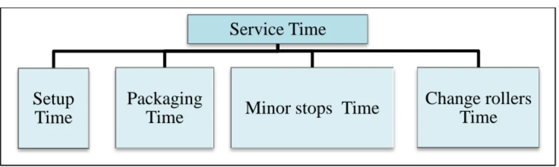
Similarly, service time analysis was necessary to avoid machines variability. Setup time, packaging time, minor stops time, and change material rollers time are the significant factors of service time as shown in figure 4.4.
Figure 4.4: Service Time factors.
4.3.2.1 Setup time study:
Setup time study was classified into two stages average setup time per item and average quantity per each item to get the average setup time per unit. Each item has different dimensions and some order has same item name which means same machine setup.
Firstly, 44 random observations for setup time were taken between all machines then a histogram with a normal curve drawn for all observations. One observation was an outlier because of a maintenance problem so this observation is neglected. Otherwise; all the other observations has a normality distribution with mean equal 10.46 minutes, median equal 10 minutes and mode equal 10 minutes –all observations data and graphs will be presented in Appendix A.6. Median was preferable to use as the average setup time per item which is 10 minutes.
Secondly, due to the lack of data for cutting machines; 2,009 different orders for daily finished products for printing machines data –November 2017- had been used to calculate the average quantity per each item. Assuming that all daily finished products from printing machines goes directly to cutting machines at same day. Daily data, number of items per day, average daily setup time and average setup time per unit are shown in Appendix A.6 with the histogram with normal curve graph for the average daily setup time to show the
Service Time
Packaging
Time Minor stops Time
Change rollers Time Setup
27
normality of data. Average setup time per unit was calculated by taking the daily average setup time per unit during the month which is equal 0.45 minutes.
4.3.2.2 Packaging Time Study:
Packaging time classified into two factor first one is the average time for packing one packet and the second factor is how many packets needed for each unit (equation 4.1). Firstly, 100 random observations had been used to find the average time needed for packing packet. Median was preferable to use as the average time needed for packet which is 0.5 minutes. All observations data and histogram with normal curve will be presented in Appendix A.7 which shows the normality of data.
Secondly, 2208 different order data with over all 10,758,232 products quantity during November 2017 had been used to get the average needed packets per unit; weighted average method for packing time had been used (equation 4.2)- to increase results accuracy as shown in tables (4.3), (4.4):
Table 4.3: Orders Classification and Quantity Percentage. Order Quantity pieces Average packet
capacity Quantity Quantity % Order > 2,000 100 pieces 946,191 8.795 % 2,000 < order ≤ 4,000 400 pieces 886,306 8.238 % 4,000 < order ≤ 15,000 1,500 pieces 3,485,656 32.399 % 15,000 < order 4,000 pieces 5,440,079 50.566 % capacity packet average unit per pieces unit per packets of Number (4.1) Table 4.4: Number of Packets needed per unit.
Order Quantity pieces Average packet capacity
number of packets per unit
Order > 2,000 100 pieces 10
2,000 < order ≤ 4,000 400 pieces 2.5 4,000 < order ≤ 15,000 1500 pieces 0.67
28 (4.2)
4.3.2.3 Minor Stops Time Study:
Firstly, forty six random observations had been used to experiment the normality of the observations results, then the mean of the observation consider as the average minor stops time = 0.8811 min/unit. Observations data and graph will be presented in Appendix A.8. 4.3.2.4 Change Rollers Time Study:
Change material roller time per unit consider two factors; time for change and number of rollers per unit (equation 4.3). Firstly, fifty random observations for change roll had been taken distributed between all machines; normality check has been done using histogram with normal curve as will be presented in Appendix A.9. Median value was preferable to us as the average time for change which is 0.5 minutes. Average changing roller time per unit has been calculated according to (equation 4.4).
length roll average unit × length production average = unit per rollers of Number (4.3) = 0.279 min/unit
29
Average service time = Setup time + Packaging time + Minor stops time + Changing roll time
Average service time = 0.45 + 0.715 + 0.8811 + 0.279 = 2.325 min/unit
4.3.3 Revised Method for Allocating The Optimum Number of Similar Machines to Operators Application:
Necessary data for revised method classified into three stages; firstly, run time and service time analysis and time study which had been discussed in section (4.3.1) and (4.3.2) and concluded in table (4.5). Secondly, financial data which has been collected by the SML’s financial department according to the monthly financial reports for year 2017 as shown in table (4.6). Final stage will be discussed in section (4.3.3.1) which is the method application.
Table 4.5: Run Time and Service Time Ratio. Average run time min/unit T = 6.81 Average service time min/unit t = 2.325
Ratio ρ = t/T = 0.34
Table 4.6: Financial Data.
Hourly fixed cost of one machine CM1 = 13.84 TL Hourly variable cost of one machine CM2 = 31.25 TL
Hourly operator cost C = 250 TL
Average material cost/unit V = 9.62 TL Average Selling price/unit L = 62.62 TL
4.3.3.1 Optimum Number of Machines to Operator:
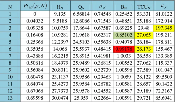
Table (4.7) demonstrates the necessary calculations for computation the optimum number of machines run by operator (N*) for both objectives minimizing cost TCUN and
maximizing hourly profit
N. The values of PtMI
,N
calculated according to Appendix A.1; HN calculated according to equation (2.6); the machine utilization N calculated according to equation (2.8); the yield per hour is QN = 60 × N/HN units equation (2.7); the30
workloads BN were calculated according to equation (2.9); TCUN calculated according to
equation (2.10); and the average hourly profits per machine
N were calculated according to equation (2.10).Table 4.7: TCU and Hourly Profit.
N PtMI
,N
HN QN N BN TCUN
N 1 0 9.135 6.56814 0.74548 0.25452 53.331 61.0122 2 0.04032 9.5188 12.6066 0.71543 0.48851 35.188 172.914 3 0.09338 10.0759 17.8644 0.67587 0.69225 29.48 197.345 4 0.16408 10.9281 21.9618 0.62317 0.85102 27.065 195.211 5 0.25366 12.2397 24.5103 0.55638 0.94978 26.184 178.611 6 0.35056 14.066 25.5937 0.48415 0.99176 26.173 155.467 7 0.43686 16.2215 25.8915 0.41981 1.0033 26.558 133.385 8 0.50616 18.4979 25.9489 0.36815 1.00552 27.062 115.337 9 0.56084 20.8011 25.9602 0.32739 1.00596 27.589 101.047 10 0.60478 23.1137 25.9586 0.29463 1.0059 28.122 89.5509 11 0.64074 25.4273 25.9564 0.26782 1.00581 28.657 80.1422 12 0.67066 27.7373 25.9578 0.24552 1.00587 29.189 72.3167 13 0.69598 30.0474 25.959 0.22664 1.00591 29.721 65.6941Table 4.7 shows that the optimum number of machines to be assigned to one operator for
minimizing cost TCUN is N* = 6 and for maximizing hourly profit
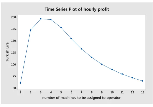
N is N* = 3. Moreover, according to the other constrains work load per worker should not be more that 85 percent so N* for minimizing cost would be equal 4.Figure (4.5) and (4.6) shows the sensitive change for maximizing profit and minimizing cost by changing the number of machines to be operates per operator. Machine utilization and work load graphs presented in Appendix A.10.
31
Figure 4.5: Hourly Profit per Machine for one Operator and N Machines
Figure 4.6: TCU for one Operator and N Machines
13 12 11 10 9 8 7 6 5 4 3 2 1 200 175 150 125 100 75 50
number of machines to be assigned to operator
Tu rk is h Li ra
Time Series Plot of hourly profit
13 12 11 10 9 8 7 6 5 4 3 2 1 55 50 45 40 35 30 25
number of machines to be assigned to operator
Tu rk is h Li ra
32 4.3.3.2 Optimum number of operators:
Distributing the total number of cutting machines inside the department to match with the optimum number of machines to be assigned to one operator (N*) to get the optimum number of operators to run all machines (K*).
K* for maximum profit strategy:
Total Number of machines M = 13 machine
Optimum number of machines to be assigned by one operator N* = 3 machines Number of operators K* [M/N*] = 13/3 = 4.33 which is not an integer number.
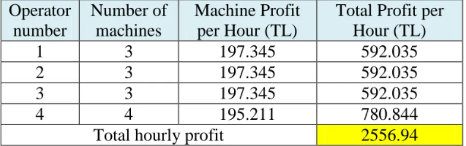
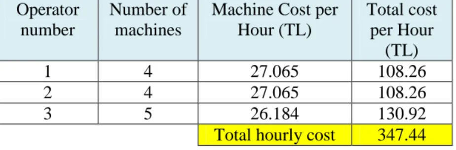
Optimum number of operator has two alternatives either to be four or five operators; to examine the two possibilities alternatives –table 4.8, 9- two steps was followed. Firstly, distribute all machines over the operators equally as much as possible with respect to assign three machines for each operator as much as possible which give the maximum hourly profit. Secondly, examine which alternative will get the maximum hourly profit to be the optimum number of operators K*. Table 4.8 shows the maximum hourly profit.
Table 4.8: Total Hourly Profit First Alternative. Operator number Number of machines Machine Profit per Hour (TL)
Total Profit per Hour (TL)
1 3 197.345 592.035
2 3 197.345 592.035
3 3 197.345 592.035
4 4 195.211 780.844
Total hourly profit 2556.94
Table 4.9: Total Hourly Profit Second Alternative. Operator number Number of machines Machine Profit per Hour (TL)
Total Profit per Hour (TL) 1 3 197.345 592.035 2 3 197.345 592.035 3 3 197.345 592.035 4 2 172.914 345.828 5 2 172.914 345.828