Selçuk J. Appl. Math. Selçuk Journal of Vol. 6. No. 2. pp. 79-98, 2005 Applied Mathematics
A Stochastic Approach to Interactive Fuzzy Multi-Objective Linear Programming for Aggregate Production Planning
Turan Paksoy1 and Mehmet Atak2
1Department of Industrial Engineering, Faculty of Engineering and Architecture, Selçuk
University, Alaaddin Keykubad Campus, Konya, Turkey; e-mail:tpaksoy@ selcuk.edu.tr;
2Department of Industrial Engineering, Faculty of Engineering and Architecture, Gazi
University, Maltepe, Ankara, Turkey; e-mail:m atak@ gazi.edu.tr;
Received: October 26, 2005
Summary. This study aims to combine probability theory and fuzzy set the-ory for solving multi-objective aggregate production planning (APP) problems. Herein, a multi-objective APP model is developed and an approach based on the interactive fuzzy linear programming is introduced to solve the APP problems that have fuzzy coe¢ cients, random demands and crisp variables. Applying the model, a decision maker can represent his/her human resources policies re-garding the overtime and subcontract production. In the following, initially, the stochastic aspect of the model is worked out. Next, the optimal solution is found by using an interactive method that decides the best compromised solu-tion among the nondominated solusolu-tion sets at each step. Finally, a numerical example is presented to clarify the features of the proposed approach.
Key words: Multi-Objective Linear Programming, Interactive Programming, Fuzzy Parameters, Stochastic Approach, Aggregate Production Planning.
1. Introduction
Linear programming problems are to optimize (maximize or minimize) an ob-jective function under some constraints. In conventional linear programming elements of problem are assumed to be crisp. However, in real world problems, constraints and objective functions are fuzzy. Therefore, while solving real-life problems, decision makers must face the di¢ culty of quantifying linguistic or
vague information. In fact, this fuzzy information represents subjective knowl-edge. Decision makers (DM) mostly make di¤erent assumptions on the models. Among the assumptions made by the DMs, vague information is very often ig-nored. On the other hand, wide ranges of production planning problems are characterized by uncertainty and ambiguity in the manufacturing industry. Since the …rst paper on fuzzy was introduced by Zadeh [31], several kinds of fuzzy linear programming models have emerged in the literature [2, 3, 5, 13], especially in the last few years [1, 15, 16, 17]. Now, several kinds of areas exist, where fuzzy linear programming is applied, [4, 11, 12, 19, 25]. One of these areas is aggregate production planning (APP). In the past several decades, a variety of deterministic and/or fuzzy models have been developed to solve APP problems [8, 10, 18, 27, 28, 29].
The term “aggregate” represents the planning made for two or more produc-tion categories. The purpose of APP is to determine producproduc-tion levels in all categories for matching recent ‡uctuating or uncertain demands. In order to achieve this aim, APP considers hiring, …ring, over time, backordering, subcon-tracting, inventory levels and the other elements of system to be modeled. It also determines appropriate sources for production. Unlike the general practice, when using APP models, inputs of the model such as sources, demands, and costs are assumed to be constant/crisp.
In this paper, an APP model is developed that lets the DM represent his/her human resources, overtime and subcontract production policies mathematically. Further, a stochastic approach to interactive fuzzy multi-objective linear pro-gramming for the APP model is introduced. In the proposed approach, initially, stochastic aspect of the model is worked out. Then the best-compromised lution among the nondominated solution sets, which are obtained from the so-lution of the multi-objective linear programming problem, is decided using an interactive method. Also, the proposed method calculates the weights of each objective function by pairwise comparisons based on Analytic Hierarchy Process (AHP).
This study is organized in six sections. After the introduction, where the aim and the scope of the study are described, the paper is structured as follows: In section 2, the developed multi-objective APP model is presented and compared to earlier proposals in the literature. The proposed approach is introduced in Section 3. Section 4 illustrates working principle of the approach on a numerical example. The results of the numerical example are discussed in Section 5 and the whole work is concluded inSection 6.
2. Interactive Fuzzy Multi-Objective Linear Programming for Ag-gregate Production Planning
Interactivity for solving fuzzy multi-objective linear programming problems has received considerable attention [7, 14, 21, 23, 26, 30]. As part of this attention,
Sasaki and Gen’s (S-G) method [24] is the one that speci…es the best com-promised solution among the nondominated solution set. This solution set is gathered from the solution of the multi-objective linear programming (MOLP) problem. Also, S-G method enlightens the structure of the DM’s preference through the conversations with the DM repeatedly.
Vagueness and multi-objectiveness are common characteristics of most decision-making processes to be modeled. However, interactivity has also as much of an importance. Thus, Sasaki and Gen’s method uses Analytic Hierarchy Process (AHP) and runs interactively, giving weights to objectives through preemptions of user. In order to …nd the best solution in the fuzzy environment, their method interacts continuously in the solution phase.
Paksoy and Atak [20] adapted the multi-objective aggregate production plan-ning model with fuzzy parameters, which is proposed by Gen et al. [10], to an industrial plant. They reached the solution by using the S-G interactive multi-objective linear programming method. Here, we develop a multi-multi-objective APP model and propose a fuzzy-stochastic approach based on the S-G method to solve it.
2.1. Modeling of Problem
In this section, based on Gen et al. [10], an APP model is developed. The construction of mathematical model requires the de…nition of the following el-ements: objectives, decision variables, constants, parameters, costs, demands, work force levels and the several other assumptions.
Minimize total production cost (Z1)
(1) min Z1= T X t=1
fcpt(prt + pot) + cst:pst+ (crt:wt) + (cot :k:pot)g
Minimize total inventory and backorder cost (Z2)
(2) min Z2=
T X t=1
fcit:it + cbt:btg
Minimize labor hiring level (Z3)
(3) min Z3=
T X t=1
fhtg
Minimize labor …ring level (Z4)
(4) min Z4=
T X t=1
Four objective functions (Z1; Z2; Z3; Z4) are considered, where: Decision variables:
prt = regular time production in period t (units) pot = over time production in period t (units) pst = subcontract production in period t (units)
wt = work force level in period t (man-day)
it = inventory level in period t (units)
bt = backorder level in period t (units)
ht = worker hired in period t (man-day)
ft = worker …red in period t (man-day)
Constants:
cpt = production cost except for labor cost in period t (TL=Turkish money/unit)
cst = cost to subcontract one unit of product in period t (TL/unit)
cot = overtime labor cost in period t (TL/man-hour) crt = labor cost in period t (TL/man-day)
cit = inventory carrying cost in period t (TL/unit-period) cbt = stockout cost in period t (TL/unit-period)
wtmax = maximum work force available in period t (man-day) Dt = forecasted demand in period t (units)
Dtmin = minimum demand in period t (units)
T = planning horizon
i0 = initial inventory level (units)
w0 = initial work force level (man-day)
b0 = initial backorder level (units)
Parameters:
k = conversion factor in hours of labor per unit of production = regular time per worker (man-hour/man-day)
= fraction of subcontract production allowable
= fraction of working hours available for overtime production = fraction of labor hiring allowable for variation
= fraction of labor …ring allowable for variation
In this model, cpt, cst, cot, crt; wtmax; Dt; , , , are assumed to be fuzzy numbers which have triangular membership function.
Constraints:
For each period, the following constraints apply:
(5) wt wt max 8t
(7) ht wt 1: t 8t; (8) ft wt 1: t 8t; (9) k:prt :wt 8t; (10) k:pot t: :wt 8t; (11) pst t(prt+ pot) 0 8t; (12) prt+ pot+ pst+ it 1 bt 1 Dt min 8t; (13) it bt= it 1 bt 1+ prt+ pot+ pst Dt 8t; (14) prt; pot; pst; wt; it; bt; ht; ft 0 8t;
The work force should not be greater than the maximum available level during any period (5). The work force in period t should equal to the work force in period t 1 plus the new hires minus the …res (6). The variation of work force level should not exceed the permitted level of company’s policy during any period (7), (8). The regular time and over time production should not be greater than the available labor capacity (9), (10). The subcontracted production should not be greater than permitted percentage of the sum of regular and over time production (11). Total production level (regular, overtime and subcontracted production) in period t plus inventory level minus backorder level in period t 1 should be greater than or equal to the minimum demand (12). In the same period, it is not allowed to be both in inventory and on backorder.
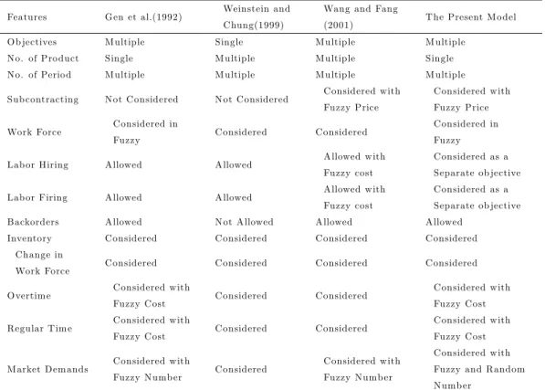
2.2 A Comparative Analysis
In order to clarify the di¤erences between our model and some others, a com-parative table adapted from Wang and Fang [28] is presented below.
Features G en et al.(1992) Weinstein and C hung(1999)
Wang and Fang
(2001) T he Present M o del
O b jectives M ultiple Single M ultiple M ultiple
N o. of Pro duct Single M ultiple M ultiple Single
N o. of Perio d M ultiple M ultiple M ultiple M ultiple Sub contracting N ot C onsidered N ot C onsidered C onsidered w ith
Fuzzy Price
C onsidered w ith Fuzzy Price Work Force C onsidered in
Fuzzy C onsidered C onsidered
C onsidered in Fuzzy Lab or H iring A llowed A llowed A llowed w ith
Fuzzy cost
C onsidered as a Separate ob jective Lab or Firing A llowed A llowed A llowed w ith
Fuzzy cost
C onsidered as a Separate ob jective
Backorders A llowed N ot A llowed A llowed A llowed
Inventory C onsidered C onsidered C onsidered C onsidered C hange in
Work Force C onsidered C onsidered C onsidered C onsidered
O vertim e C onsidered w ith
Fuzzy C ost C onsidered C onsidered
C onsidered w ith Fuzzy C ost R egular T im e C onsidered w ith
Fuzzy C ost C onsidered C onsidered
C onsidered w ith Fuzzy C ost
M arket D em ands C onsidered w ith
Fuzzy N umb er C onsidered
C onsidered w ith Fuzzy N umb er
C onsidered w ith Fuzzy and R andom N umb er
Table 1 A comparative analysis table for APP models
3. Stochastic Approach to the Problem
In the model given in Section 2, minimum demands (Dtmin) are considered as normally distributed random numbers. A method, introduced by Chalam [6], is used to manage the stochastic aspect of the model. Initially, the model is solved by using this method, so that the stochastic environment could be avoided. Second, the S-G interactive method is applied.
The following stochastic-fuzzy hybrid linear programming problem is treated
M axZk= n X J =1 CkjXj; k = 1; 2; :::q1 M inZk= n X J =1 CkjXj; k = q1+ 1; :::q2 s:t : Xn j=1aijXj~ bi; i = 1; 2; :::m1 Xn j=1aijXj bi; i = m1+ 1; :::m2
Xn
j=1aijXj bi; i = m2+ 1; :::m3 Xn
j=1aijXj= bi; i = m3+ 1; :::m
(15) Xj 0; j = 1; 2; :::n
where; Ckj = (Ckj1; Ckj2; Ckj3) is a fuzzy coe¢ cient of the kth objective func-tion and jth decision variable,
biis a vector of random right hand sides which have normal distribution function and ~ is “fuzzi…ed version of ” having the linguistic interpretation “approxi-mately greater than or equal” for i = 1; 2; :::m1.
aij= (aij1; aij2; aij3)is a fuzzy technical coe¢ cient of the ith constraint and the jth decision variable for i = m1+ 1; :::m,
bi = (bi1; bi2; bi3)is a fuzzy right hand side of the ith constraint for i = m1+ 1; :::m.
When fuzzy numbers are used in this paper, it is assumed that they have trian-gular membership function. Such a number ~f , can be shown as ~f = (f1; f2; f3) and its membership function is as follows (See Fig. 1).
(16) f~(x) = 8 < : 1 f2 f1(x f2) + 1 ; (f1 x f2 1 f2 f3(x f2) + 1 ; (f2 x f3) 0 ; (x f1; f3 x)
Figure 1. A Triangular Fuzzy Numberf~
Here, in order to solve with the S-G interactive method, a two-stage approach is proposed for preparing the problem (15)
In the …rst stage, using the method proposed by Gen et al. [10], the model is taken out of fuzziness except for the constraints with random right hand sides and reformulated as follows.
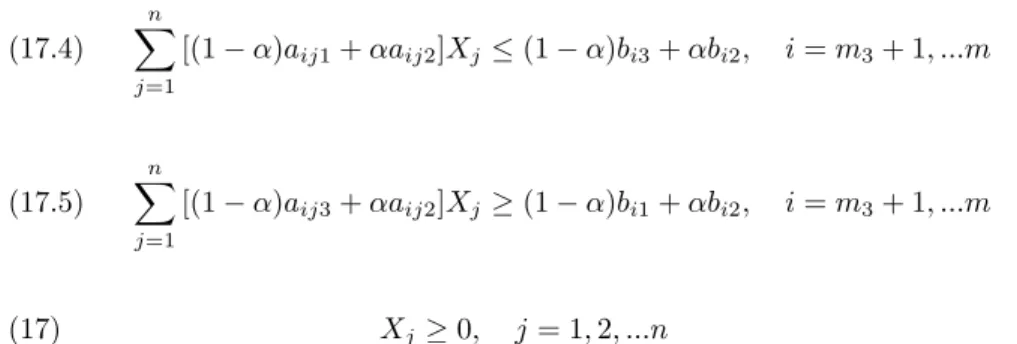
M axZk= n X j=1 [(1 )Ckj3+ Ckj2]Xj; k = 1; 2; :::q1 M inZk= n X j=1 [(1 )Ckj1+ Ckj2]Xj; k = q1+ 1; :::q2 s:t : (17.1) Xn j=1aijXj~ bi; i = 1; 2; :::m1 (17.2) n X j=1 [(1 )aij1+ aij2]Xj (1 )bi3+ bi2; i = m1+ 1; :::m2 (17.3) n X j=1 [(1 )aij3+ aij2]Xj (1 )bi1+ bi2; i = m2+ 1; :::m3
(17.4) n X j=1 [(1 )aij1+ aij2]Xj (1 )bi3+ bi2; i = m3+ 1; :::m (17.5) n X j=1 [(1 )aij3+ aij2]Xj (1 )bi1+ bi2; i = m3+ 1; :::m (17) Xj 0; j = 1; 2; :::n
where, is a cuto¤ value such that 0 < < 1. For fuzzi…ed constraints (Eq. 17.1), it is assumed that bi is a random variable which has normal distribution function Ni, i = 1; 2; :::m1.
bi may be considered as the average value of Di i.e., E(Di)=bi, i = 1; 2:::m1. bi N ( i; i);the density function of bi is
(18) f (bi; ; ) = ( 1 p 2 e (bi )2 2 2 ; 1 < bi< 1 0 ; otherwise
where i represents the standard deviation of Di and i is the mean (See Fig. 2).
Figure 2. P f n < x < + n gforn = 1; 2; 3
In the problem (17), bi= (b1; b2; :::bm1) is a vector of random numbers normally distributed and for these right hand sides as seen in the Fig. 2, the decision area is split into three parts; j , 2 j and 3 j bounds.
Let Ai be the fuzzy set corresponding to the ith constraint in the Eq. (17.1). Following Zimmermann [32], the membership function of Ai can be de…ned as,
(19) i= 8 > < > : 1P if Pnj=1aijXj bi n j=1aijXj bi bi bi if bi < Pn j=1aijXj< bi 0 if Pnj=1aijXj bi where bi is the lower tolerance limit of Pnj=1aijXj.
For bi, Chalam [6] proposes to try bi i…rst. If a nonfeasible situation exists, we relax bi by taking bi 2 i. If we still cannot achieve the feasibility, relax bi further by bi 3 i.
In fuzzy decision-making, the overall decision function D can be de…ned by the intersection operator as D = \n
j=1Ai: The membership function of D becomes,
(20) D=
n ^ j=1
Ai = M in Ai
The crisp equivalent of (17) can now be de…ned as,
(21) M ax D Subject to; D Ai; i = 1; 2; :::; m1 Eqs. (17.2)-(17.5), i = m1+ 1; :::; m; Xj 0; j = 1; 2; :::; n: Let = M in i " Pn j=1aijXj bi bi bi #
and formulate the above problem as an equiv-alent linear programming problem as,
(22) M ax Subject to; " Pn j=1aijXj bi bi bi # ; i = 1; 2; :::; m1 Eqs. (17.2)-(17.5), i = m1+ 1; :::; m; ; Xj 0; j = 1; 2; :::; n:
The traditional linear programming model (22) can be solved easily. Following Chalam [6], initially take bi as (bi i). In case of nonfeasibility relax its value by taking bi = bi 2 i and if still found nonfeasible further relax it by bi = bi 3 i.
Now, we substitute into the model and determine the new right hand sides of Eq. (17.1) (minimum demands) as follows:
M axZk = n P j=1 [(1 )Ckj3+ Ckj2]Xj; k = 1; 2; :::q1 M inZk = n P j=1 [(1 )Ckj1+ Ckj2]Xj; k = q1+ 1; :::q2 Subject to: (23) Pn j=1aijXj bi + (bi bi); i = 1; 2; :::m1 Eqs. (17.2)-(17.5), i = m1+ 1; :::m; ; Xj 0; j = 1; 2; :::n:
At the second stage, above, a fuzzy method is applied to release the stochastic aspect of the model and a crisp multi-objective linear programming model (23) is achieved. Finally, maintaining fuzzy thinking, the S-G interactive fuzzy method is employed. This procedure is presented in the algorithm below.
Step 1 Formulate the APP model.
Step 2 Determine the weights of objective functions using AHP and cut level Step 3 Use the method proposed by Gen et al. [10] to transform the fuzzy coe¢ cients of the model to crisp ones.
Step 4 Release the stochastic aspect of the model. Step 5 Solve the model with S-G method.
4. Numerical Example
As the illustration of the proposed approach, a sample model for aggregate production planning with six term planning horizon was solved. The solution procedure as follows:
Step 1: Formulate the APP model.
min Z1= 6 P t=1f(130000; 136000; 142000)(prt+pot)+(160000; 164000; 168000)p st+ (9200; 10000; 10800)wt + (1700; 1800; 1900):5potg min Z2= 6 P t=1f7500it + 36250btg min Z3= 6 P t=1fhtg min Z4= 6 P t=1fftg
s:t: w1 (650; 700; 750) w1 w0 h1+ f1= 0 h1 w0:(0:10; 0:20; 0:30) w2 (650; 750; 850) w2 w1 h2+ f2= 0 h2 w1:(0:10; 0:20; 0:30) w3 (650; 800; 950) w3 w2 h3+ f3= 0 h3 w2:(0:10; 0:20; 0:30) w4 (650; 800; 950) w4 w3 h4+ f4= 0 h4 w3:(0:10; 0:20; 0:30) w5 (650; 800; 950) w5 w4 h5+ f5= 0 h5 w4:(0:10; 0:20; 0:30) w6 (650; 800; 950) w6 w5 h6+ f6= 0 h6 w5:(0:10; 0:20; 0:30) f1 w0:(0:10; 0:20; 0:30) 5pr1 8w1 0 5po1 (0:10; 0:30; 0:50):8w1 0 f2 w1:(0:10; 0:20; 0:30) 5pr2 8w2 0 5po2 (0:10; 0:30; 0:50):8w2 0 f3 w2:(0:10; 0:20; 0:30) 5pr3 8w3 0 5po3 (0:10; 0:30; 0:50):8w3 0 f4 w3:(0:10; 0:20; 0:30) 5pr4 8w4 0 5po4 (0:10; 0:30; 0:50):8w4 0 f5 w4:(0:10; 0:20; 0:30) 5pr5 8w5 0 5po5 (0:10; 0:30; 0:50):8w5 0 f6 w5:(0:10; 0:20; 0:30) 5pr6 8w6 0 5po6 (0:10; 0:30; 0:50):8w6 0 ps1 (0:05; 0:10; 0:15)(pr1+ po1) 0 pr1+ po1+ ps1+ i0 b0~ N(1505; 15) ps2 (0:05; 0:10; 0:15)(pr2+ po2) 0 pr2+ po2+ ps2+ i1 b1~ N(1620; 10) ps3 (0:05; 0:10; 0:15)(pr3+ po3) 0 pr3+ po3+ ps3+ i2 b2~ N(1360; 10) ps4 (0:05; 0:10; 0:15)(pr4+ po4) 0 pr4+ po4+ ps4+ i3 b3~ N(1310; 20) ps5 (0:05; 0:10; 0:15)(pr5+ po5) 0 pr5+ po5+ ps5+ i4 b4~ N(1340; 10) ps6 (0:05; 0:10; 0:15)(pr6+ po6) 0 pr6+ po6+ ps6+ i5 b5~ N(1325; 15) i1 b1= i0 b0+ pr1+ po1+ ps1 (1520; 1550; 1580) i2 b2= i1 b1+ pr2+ po2+ ps2 (1620; 1640; 1660) i3 b3= i2 b2+ pr3+ po3+ ps3 (1380; 1410; 1440) i4 b4= i3 b3+ pr4+ po4+ ps4 (1290; 1330; 1370) i5 b5= i4 b4+ pr5+ po5+ ps5 (1340; 1390; 1440) i6 b6= i5 b5+ pr6+ po6+ ps6 (1310; 1360; 1410) w0= 850 i0= 0 b0= 0 (24) prt; pot; wt; it; bt; ht; ft 0
The numerical example (24) has some conditions and assumptions. Initially inventory and backorders are not considered. The backorders should not be carried-over for more than one period. There is a six-period planning horizon (T ), and the initial work force level consists of 850 man-day/period. The regular time per worker ( ) is 8 hours. Overtime production is limited to 30% of regular time production ( t= 0:10; 0:30; 0:50). Subcontract and employment policy of …rm are re‡ected by following parameters respectively t = (0:05; 0:10; 0:15), t= (0:10; 0:20; 0:30), t= (0:10; 0:20; 0:30). It takes 5 hours to build one unit of product for a worker (k = 5).
For simplicity, …nancial values are used by omitting the last three zeros through the evaluation process. The currency parity provided by the Turkish Central Bank (TCMB) on April 12, 2005 was 1 USD= 1,344,000 TL. In the example, cpt= (130; 000; 000; 136; 000; 000; 142; 000; 000)
cst= (160; 000; 000; 164; 000; 000; 168; 000; 000) TL/unit crt = (9; 200; 000; 10; 000; 000; 10; 800; 000) TL/man-day cot = (1; 700; 000; 1; 800; 000; 1; 900; 000) TL/man-hour cit= 7; 500; 000, cbt= 36; 250; 000 TL/unit-period
Step 2: Determine the weights of objective functions and cut level
Step 2.1 : In this step, Analytic Hierarchy Process (AHP), proposed by Saaty [22], is used. AHP is a powerful tool that helps the DM recognize the decision mechanism and makes it easier to choose the best alternatives.
Step 2.1.1 : Using Saaty’s pairwise comparison scale (Table 2), determine the relative weights of the set of objectives with respect to each other and express them in a pairwise comparison matrix.
Im p ortance/
Preference Level Verbal D e…nition Explanation
1 Equal im p ortence of b oth elem ents
T wo elem ents contribute equally
3 M o derate im p ortance of one elem ent over another
T he D M favors one elem ent over another 5 Strong im p ortance of one
elem ent over another
T he D M favors one elem ent strongly 7 Very strong im p ortance of
one elem ent over another
A n elem ent is very strongly dom inant 9 Extrem e im p ortance of
one elem ent over another
A n elem ent is extrem ely dom inant
2,4,6,8 Interm ediate values U sed to com prom ise b etween two judgm ents
Table 2 Pairwise Comparison Scale used in AHP [22]
The following matrix, which is called “pairwise comparison matrix”, represents the DM’s judgment numerically.
A = 2 6 6 4 1 3 5 5 1 3 1 3 3 1 5 1 3 1 2 1 5 1 3 1 2 1 3 7 7 5
Step 2.1.2 : Divide the column elements of the comparison matrix by sum of columns and get the normalized matrix Anorm.
Anorm= 2 6 6 4 0:57692 0:64286 0:52632 0:45454 0:19231 0:21429 0:31579 0:27273 0:11538 0:07143 0:10526 0:18182 0:11538 0:07143 0:05263 0:09091 3 7 7 5
Step 2.1.3 : Calculate the row averages of the normalized matrixAnormand get the weight column matrix WT.
w1= (0:57692 + 0:64286 + 0:52632 + 0:45454)=4 = 0:55016 w2= (0:19231 + 0:21429 + 0:31579 + 0:27273)=4 = 0:24878 w3= (0:11538 + 0:07143 + 0:10526 + 0:18182)=4 = 0:11847 w4= (0:11538 + 0:07143 + 0:05263 + 0:09091)=4 = 0:08259 WT = 2 6 6 4 0:55016 0:24878 0:11847 0:08259 3 7 7 5
Step 2.1.4 : Evaluate the consistency.
Step 2.1.4.1 : A:WT = 2 6 6 4 1 3 5 5 1 3 1 3 3 1 5 1 3 1 2 1 5 1 3 1 2 1 : 0:55016 0:24878 0:11847 0:08259 3 7 7 5 = 2 6 6 4 2:30180 1:03535 0:47661 0:33478 3 7 7 5 Step 2.1.4.2 : Calculate [(1=n) n P i=1
(ith element of A:WT) (ith element of WT)]
1=4:[2:30180=0:55016 + 1:03535=0:24878 + 0:47661=0:11847 + 0:33478=0:08259] = 4:10554
Step 2.1.4.3 : Calculate the Consistency Index (CI). CI= [(Result of the Step 2.1.4.2 –n)/(n –1)] CI= (4.10554 –4)/ (4 –1)= 0.03518
Step 2.1.4.4 : Calculate the Consistency Ratio (CR).
Saaty [22] simulated random pairwise comparisons for di¤erent size matrices, calculating the consistency indices and arriving at an average consistency index for random judgments for each size matrix (Table 3).
D im ension of M atrix 1 2 3 4 5 6 7 8 R andom ness Index 0.00 0.00 0.58 0.90 1.12 1.24 1.32 1.41 D im ension of M atrix 9 10 11 12 13 14 15 R andom ness Index 1.45 1.49 1.51 1.48 1.56 1.57 1.59
Table 3Randomness indices for matrices having dimensions between 1-15
Consistency Ratio (CR) is the ratio of the consistency index to the average consistency index for random comparisons for a same sized matrix.
CR = CI/RI =0.03518/0.90 = 0.0391
Inconsistency ratio of about 10% or less is usually accepted. For the exam-ple, 0.0391<0.10. Therefore, the judgment of the DM can be considered as consistent.
Following AHP procedure, weights for the objectives are calculated as follow; W = 0:55016 0:24878 0:11847 0:08259
Step 2.2 : Set cut level =0.5.
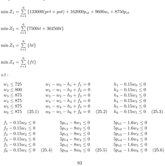
Step 3: Using the method proposed by Gen et al. [10], transform the model to LP problem with crisp coe¢ cients
min Z1= 6 P t=1f133000(prt + pot) + 162000pst + 9600wt+ 8750pot min Z2= 6 P t=1f7500it + 36250btg min Z3= 6 P t=1fhtg min Z4= 6 P t=1fftg s:t : w1 725 w2 800 w3 875 w4 875 w5 875 w6 875 (25.1) w1 w0 h1+ f1= 0 w2 w1 h2+ f2= 0 w3 w2 h3+ f3= 0 w4 w3 h4+ f4= 0 w5 w4 h5+ f5= 0 w6 w5 h6+ f6= 0 (25.2) h1 0:15w0 0 h2 0:15w1 0 h3 0:15w2 0 h4 0:15w3 0 h5 0:15w4 0 h6 0:15w5 0 (25.3) f1 0:15w0 0 f2 0:15w1 0 f3 0:15w2 0 f4 0:15w3 0 f5 0:15w4 0 f6 0:15w5 0 (25.4) 5pr1 8w1 0 5pr2 8w2 0 5pr3 8w3 0 5pr4 8w4 0 5pr5 8w5 0 5pr6 8w6 0 (25.5) 5po1 1:6w1 0 5po2 1:6w2 0 5po3 1:6w3 0 5po4 1:6w4 0 5po5 1:6w5 0 5po6 1:6w6 0 (25.6)
ps1 0:075(pr1+ po1) 0 ps2 0:075(pr2+ po2) 0 ps3 0:075(pr3+ po3) 0 ps4 0:075(pr4+ po4) 0 ps5 0:075(pr5+ po5) 0 ps6 0:075(pr6+ po6) 0 (25.7) pr1+ po1+ ps1+ i0 b0~ N(1505; 15) pr2+ po2+ ps2+ i1 b1~ N(1620; 10) pr3+ po3+ ps3+ i2 b2~ N(1360; 10) pr4+ po4+ ps4+ i3 b3~ N(1310; 20) pr5+ po5+ ps5+ i4 b4~ N(1340; 10) pr6+ po6+ ps6+ i5 b5~ N(1325; 15) (25.8) i0 b0 i1+ b1+ pr1+ po1+ ps1 1565 i1 b1 i2+ b2+ pr2+ po2+ ps2 1650 i2 b2 i3+ b3+ pr3+ po3+ ps3 1425 i3 b3 i4+ b4+ pr4+ po4+ ps4 1350 i4 b4 i5+ b5+ pr5+ po5+ ps5 1415 i5 b5 i6+ b6+ pr6+ po6+ ps6 1385 (25.9) i0 b0 i1+ b1+ pr1+ po1+ ps1 1535 i1 b1 i2+ b2+ pr2+ po2+ ps2 1630 i2 b2 i3+ b3+ pr3+ po3+ ps3 1395 i3 b3 i4+ b4+ pr4+ po4+ ps4 1310 i4 b4 i5+ b5+ pr5+ po5+ ps5 1365 i5 b5 i6+ b6+ pr6+ po6+ ps6 1335 (25.10) w0= 850 i0= 0 (25.11) b0= 0 (25) prt; pot; wt; it; bt; ht; ft 0
Step 4: Release the stochastic aspect of the model.
First of all, the mean values of the random variables (Dtmin) are taken to solve the model. However, with these values (1505; 1620; 1360; 1310; 1340; 1325) the model has no feasible solution. Consequently, they must be relaxed by j. In this case, the problem becomes as follows.
max s:t : Eqs. (25.1)-(25.7) pr1+ po1+ ps1+ i0 b0 15 1490 pr2+ po2+ ps2+ i1 b1 10 1610 pr3+ po3+ ps3+ i2 b2 10 1350 pr4+ po4+ ps4+ i3 b3 20 1290 pr5+ po5+ ps5+ i4 b4 10 1330 pr6+ po6+ ps6+ i5 b5 15 1310
Eqs. (25.9)-(25.11)
(26) prt; pot; wt; it; bt; ht; ft; 0
To solve this model, an optimization software (LINDO) was used and a feasible solution at = 0:26 was obtained. Now, we substitute into the model and de-termine the new right hand sides of Eq. (25.8) as follows: 1493:9; 1612:6; 1352:6; 1295:2; 1332:6; 1313:9:
Step 5: Solve the model by S-G method. (f1; f1 ) = (1194690000; 1462717000) (f2; f2 ) = (2029999; 99999900) (f3; f3 ) = (75; 625)
(f4; f4 ) = (125; 641:25)
Goal values (hk) for each objective function are set from the following range by the DM: fk hk fk, k = 1; 2; ::4. And let DM choose goals near the best values as: (1195000000; 2500000; 75; 125):
Following results are obtained by using the algorithm: Z1= 1195463475; Z2= 2794875; Z3= 75; Z4= 125
wt= (725; 800; 800; 800; 800; 800); prt= (1160; 1280; 1280; 1280; 1280; 1280) pot= (232; 256; 132:4; 30; 85; 33:9); pst= (104:4; 115:2; 0; 0; 0; 0)
ht= (0; 75; 0; 0; 0; 0); ft= (125; 0; 0; 0; 0; 0); it= (0; 0; 0; 0; 0; 0; 0) bt= (0; 38:6; 17:4; 0; 0; 0; 21:1)
5. Results and Discussions
The numerical example applied had constraints on a large scale for imitating real world problems. Thus, the results achieved by using the method in the example can be treated as expressive data for assessing the e¢ ciency of the approach. The results can be formulated in a general way as follows: the method speci-…es about the total production cost, inventory levels, over time, backordering, subcontracting levels, labor hiring and …ring levels.
The decision maker, who chooses the goal values for the objective functions, a¤ects the solution through his preference structure. In addition to this con-structive e¤ect, the method including the fuzziness and randomness does not allow the simpli…cation of the certainty assumptions to limit the validity of the results.
Using the preferred goal values (1195000000; 2500000; 75; 125, in the exam-ple), a compromise solution is obtained. The results show that, total produc-tion cost and total inventory and backorder cost for the next six months are 1,195,463,475,000 TL and 2,794,875,000 TL respectively. Labor hiring level is 75 man-day and labor …ring level is 125 man-day for the planning horizon. For the …rst month, proposed work force level is 725 man-day, and then, with a 75 man-day hiring, 800 man-day level until the end of horizon.
The production plan suggests 1160 units regular time production, 232 units overtime production, 104.4 units subcontract production, a total of 1496.4 units production for the …rst month; 1280 units regular time production, 256 units overtime production, 115.2 units subcontract production, a total of 1651.2 units production for the second month; 1280 units regular time production, 132.4 units overtime production, a total of 1412.4 units production for the third month; 1280 units regular time production, 30 units overtime production, a total of 1310 units production for the fourth month; 1280 units regular time production, 85 units overtime production, a total of 1365 units production for the …fth month; 1280 units regular time production, 33.9 units overtime production, a total of 1313.9 units production for the sixth month.
For human resources planning, the results show that except for the second month (75 man-day) no one is hired. Similarly, …ring occurs only on the …rst month (125 man-day). Certainly, the parameters re‡ecting the policy of the …rm a¤ect the formation of this solution strongly.
Inventory is also an undesirable component in the plan with zero level through the whole horizon. The backorder levels are 38.6 units for the second month, 17.4 units for the third month and 21.1 units for the sixth months.
These detailed results constitute a quite e¤ective plan for decision makers to manage the production system.
6. Conclusions
In this paper, an approach has been developed by integrating possibility and probability theory for an aggregate production planning problem. Employing the developed APP model, decision maker can represent his/her human re-sources policy and policies for the rate of overtime and subcontract production. In the solution procedure of the proposed approach, the stochastic aspect of the model is treated at …rst. Second, the best-compromised solution among the nondominated solution sets is decided through the conservations with the DM repeatedly. A numerical example is presented to clarify the features of the proposed approach.
The purpose of the paper is to introduce a new fuzzy-stochastic approach, where normally distributed random variables are transferred into triangular fuzzy num-bers. The approach based on the interactive fuzzy linear programming is in-tended to solve multi-objective aggregate production planning problems with
fuzzy coe¢ cients, random demands and crisp variables. Proposed approach mentions the advantages of considering both fuzzy and probabilistic nature. Thus, this combining approach is more successful to re‡ect the real world. Notwithstanding the above merits mentioned, the proposed approach has some points, which need to be developed as future work. For instance, fuzzy multi-objective programming method presented by Dengfeng and Chuntian [9] can be integrated to the approach or di¤erent membership functions can be used in the model. Therefore, more e¢ cient methods need to be investigated.
References
1. Bector C. R and Chandra S. (2002): On duality in linear programming under fuzzy environment, Fuzzy Sets and Systems 125(3), 317-325.
2. Bellman R. E. and Zadeh L. A. (1970): Decision Making in a Fuzzy Environment, Management Science 17, 8141-8164.
3. Buckley J. J. and Feuring T. (2000): Evolutionary algorithm solution to fuzzy problems: Fuzzy linear programming, Fuzzy Sets and Systems 109(1), 35-53.
4. Cadenas J. M., Pelta D. A. Pelta H. R. and Verdegay J. L. (2004): Application of fuzzy optimization to diet problems in Argentinean farms, European Journal of Operational Research, 158 (1) 218-228.
5. Carlsson C. and Korhonen P. (1986): A Parametric Approach to Fuzzy Linear Programming, Fuzzy Sets and Systems 20, 17-30.
6. Chalam G. A. (1994): Fuzzy goal programming approach to a stochastic trans-portation problem under budgetary constraint, Fuzzy Sets and Systems 66, 293-299. 7. Cross V., De Cabello M. (1995): Fuzzy interactive multiobjective optimization on borrowing/lending problems, Proceedings of 3rd Int. Symposium on Uncertainty Modeling and Analysis and Annual Conf. of the North American Fuzzy Inf. Processing Soc., 513-518.
8. Das B. P., Rickard J. G., Shah N. and Macchietto S. (2000): An investigation on integration of aggregate production planning, master production scheduling and short-term production scheduling of batch process operations through a common data model, Computers and Chemical Engineering 24, 1625-1631.
9. Dengfeng L.and Chuntian C. (2002): Fuzzy multiobjective programming meth-ods for fuzzy constrained matrix games with fuzzy numbers, International Journal of Uncertainty, Fuzziness and Knowledge-Based Systems 10(4), 385-400.
10. Gen M., Tsujimura Y. and Ida K. (1992): Method for solving multiobjective aggre-gate production planning problem with fuzzy parameters, Computers and Industrial Engineering 23(1-4), 117-120.
11. Guo P. and Tanaka H. (2001): Fuzzy DEA: a perceptual evaluation method, Fuzzy Sets and Systems 119(1), 149-160.
12. Gupta A. P., Harboe R. and Tabucanon M. T. (2000): Fuzzy multiple-criteria decision making for crop area planning in Narmada river basin, Agricultural Systems 63(1), 1-18.
13. Herrera F. and Verdegay J. L. (1996): Fuzzy boolean programming problems with fuzzy costs: A general study, Fuzzy Sets and Systems 81(1), 57-76.
14. Hota P. K. Chakrabarti R.and Chattopadyay P. K. (2000): Economic emission load dispatch through an interactive fuzzy satisfying method, Electric Power Systems Research 54(3), 151-157.
15. Jamison K. D. and Lodwick W. A. (2001): Fuzzy linear programming using a penalty method, Fuzzy Sets and Systems 119(1), 97-110.
16. Li C., Liao X. and Yu J. (2004): Tabu search for optimization and applications, Information Sciences 158, 3-13.
17. Li D. F. and Yang J. B. (2004): Fuzzy linear programming technique for mul-tiattribute group decision making in fuzzy environments, Information Sciences 158, 263-275.
18. Masud A. S. M. and Hwang C. L. (1980): An aggregate production planning model and application of three multiple objectives decision methods, International Journal of Production Research 18, 741-752.
19. Miller W. A., Leung L. C., Azhar T. M., and Sargent S. (1997): Fuzzy produc-tion planning model for fresh tomato packing, Internaproduc-tional Journal of Producproduc-tion Economics 53(3), 227-238.
20. Paksoy T. and Atak M. (2002): Interactive fuzzy multiobjective linear program-ming for aggregate production planning: Case study of a hydraulic pump manufacturer company, Journal of the Institute of Sciences and Technology of Gazi University 15(2), 457-466 (in Turkish).
21. Ramesh R., Karwan M. H. and Zionts S. (1989): Interactive multicriteria linear programming: an extension of the method of zionts and wallenius, Naval Research Logistics 36, 321-335.
22. Saaty T. L. (1996): The Analytic Hierarchy Process, RWS Publications, Pitts-burgh.
23. Sakawa M. and Sawada K. (1994): Interactive fuzzy satisfying method for large-scale multiobjective linear programming problems with block angular structure, Fuzzy Sets and Systems 67(1), 5-17.
24. Sasaki M. and Gen M. (1993): An extension of interactive method for solving mul-tiple objective linear programming with fuzzy parameters, Computers and Industrial Engineering 25(1-4), 9-12.
25. Shih L. H. (1999): Cement transportation planning via fuzzy linear programming, International Journal of Production Economics 58(3), 277-287.
26. Tapia C. G.and Murtagh B. A. (1991): Interactive fuzzy programming with pref-erence criteria in multiobjective decision making, Comp. Operations Research 18(3) (1991) 307-316.
27. Wang R. C. and Fang H. H. (2000): Aggregate production planning in a fuzzy environment, International Journal of Industrial Engineering 7, 5-14.
28. Wang R. C. and Fang H. H. (2001): Aggregate production planning with multiple objectives in a fuzzy environment, European Journal of Operational Research 133, 521-536.
29. Weinstein L. and Chung C. H. (1999): Integrating maintenance and production de-cisions in a hierarchical production planning environment, Computers and Operations Research 26, 1059-1074.
30. Wu S. M., Huang G. H. and Guo H. C. (1997): Interactive inexact-fuzzy approach for multiobjective planning of water resource systems, Water Science and Technology 36(5), 235-242.
31. Zadeh L. A. (1965): Fuzzy Sets, Information and Control 8, 338-353.
32. Zimmermann H. J. (1978): Fuzzy Programming and Linear Programming with Several Objective Functions, Fuzzy Sets and Systems 1, 45-55.

![Table 2 Pairwise Comparison Scale used in AHP [22]](https://thumb-eu.123doks.com/thumbv2/9libnet/4732722.89790/13.918.207.662.547.800/table-pairwise-comparison-scale-used-ahp.webp)