Time series in forecasting and decision: an experiment in elman nn models

Time Series in~Forecasting

and Decision: An Experiment in

Elman NN Models

Cvetko 1. Andreeski

'

and Gkorgi M. Dimirovski"'

'

Faculty of Tourism and Hospitality Ohrid, St. Clement of Ohrid University Bitola Key Marsal Tito bb, Ohrid, MK-6000, Republic of Macedonia

E-mail: ciuuslin@,mt.net.mk

'

Department of Computer Engineering, DOGUS University, Faculty of Engineering Acibadem, Zemaet Sk. 21, Kadikoy, 81010 Istanbul, Republic of Turkey

E-mail: gdimirovski@doaus.edu.tr

'ASE Institute

-

Faculty of Electrical Engineering, SS Cyril & Methodius University MK-1000 Skopje, Republic of Macedonia

Absbocc- The paper examines the role of analytical tools inanal ysis of economic statistical data (commonly referred to as econometry) and artificial neural network (ANN) models for time series processing in forecasting, decision and control. The emphasis is put on the comparative analysis of classical econometric approach of pattern recognition (BoxJenkins approach) and neural network models, especially the class of recurrent ones and Elman ANN in particular. A comprehensive experiment in applying the latter modeling has been carried out, some specific applications software developed, and a number of benchmark series from the literature processed. This paper reports on comparison findings in favor of Elman ANN modeling, and on the use of a designed program package that encompasses routines for regression, ARlMA and ANN analysis of time series. The analysis is illustrated by two sample examples known as dimcult to model via any technique

lnder Term: Analysis of time series; decision; financial engineering; forecasting; neural networks; patterns.

I. INTRODUCTION

TIME series analysis and prediction has been successfully used for long time to support the decision making in a number of real-world non-engineering applications that emphasized their potential in socio- economic systems forecasting and control [3], [ 8 ] , [91,

[13], [14]. Classical pattern recognition has mainly been concerned with detecting systematic patterns in an array of measurements, which do not change in time (static patterns). Typical applications involve the classification

of

input vectors into one of several classes (discriminant analysis) or the approximate description of dependencies between observables (regression). These applications use linear models for

* This research is supported in part by Faculty of Tourism and Hospitality in Ohrid, Rep. of Macedonia, and in p m by Dogus University in Istanbul, Rep. of Turkey.

system dynamics identification and prediction. However, successful capturing the underlying system dynamics in economic time series, with all their features of time-variation, nonlinearity, nonstationarity and uncertainty stemming

form

the application area, seems to be an ever open problem [3], [91.

Recently the use of artificial neural-net (ANN) computing structures has considerably expanded to economic time series analysis due to their capability to capture end emulate the underlying non-linear system dynamics, as the special 2001 issue on neural networks in financial system engineering [IS] has demonstrated. For data sets in these areas appear in the form of complexity time series. The way in which ANN computing structures are employed in the analysis of time series is based on non-linear autoregressive model with exogeneous inputs. In work [4] the application of memory A N N computing structures non-linear model identification has been studied. In work [ I O ] Chen et al. have thoroughly explored the application of A N N to the problem of inflation forecasting via three classes of neural networks having different activation functions, and proved tight root mean squared error (rms) bounds on the convergence rates of ANN estimators. In the study [ 6 ] , Bastos et al. explored evolutionary design of NN for wide applications, while Doffner focused his study [ I l l on especially designed ANN for time series processing.

11. ON NEURALNET MODELSFORTIME SERIES PROCESSING

It is known that different neural networks, according to the type of mechanism to deal with time series [I I], can be used. Most neural networks have previously been defined for pattern recognition in static panems; the temporal dimension has to be supplied additionally in an appropriate way [IO]. Some

of

them are worth mentioning: layer delay without feedback (time windows); layer delay with feedback; unit delay

without feedback; unit delay with feedback (self- recurrent loops).

Io

this research the class

of

recurrent network created with adding new elements in classic neural feed-fonvard networks, which can be trained during a certain sequence

of

time, have been studied. The important feature of kind of neural networks is that they can identify dynamic systems with

no

need for more than one previous value of the input and output.

. Therefore these are capable of identifying dynamic systems with unknown order or with unknown time delay, and are known as Elman networks.

A common method for time series processing are so called (linear) state space models

[71-[9].

The assumption is that a time series can he described as a linear transformation of a timede pendent state-given through a state vector

S

:

i ( t )

=

G(t)

+E@)

(1) where C is some transformation matrix. A linear model usually describes time dependent state vector:

F ( t )

= A ? ( t - l ) + B r j ( r )

( 2 )

where A and B are matrices, and ?(t) is a noise process, just like C(t) above. The model for the state change, in this version, is basically an ARMA[I,I] process. The basic assumption underlying this model is the assumption of so-called Markov property [12]: the next sequence element in the time series can be predictedon the grounds of the state of the system producing the time series is in,

no

matter how that state was reached. In other words, all the history of the series necessary for producing a sequence element can be expressed by one state vector. Should the assumption the states are also independent on the past sequence vector holds, by neglecting the moving average term B

fi(t),

one obtains

F ( t )

AS(?

-

1)

+

Di(t

-

1).

(3) Then, basically, an equation describing Elman type of recurrent neural networks

[ I I],

depicted in Figure 1,

is

obtained.

The Elman network is in fact a multi layer perceptron (MLP) neural-net computing structure with a n additional input layer, called the state layer, which receives a copy of the activations from the hidden layer at the previous time step

via

feedback. Should

use

this network is employed for forecasting modeling, the activation vector of the hidden layer is equated with

S

,

and then the only difference to Eq. (3) is the fact that in an MLP a sigmoid activation function is applied to the input of each hidden unit

. ? ( t ) = c ~ ( A ? ( t - l ) + D . ? ( t - l ) ) .

(4)

Here a(a) refers to the application of the sigmoid (or logistic) function I/(l+exp(-aJ)

to

each element a;

of

A. Hence the transformation is no longer linear but a non-linear one according to the logistic regressor applied to the input vectors.

Fig. I . The smcNre of Elman neural-networks

The Elman network can be trained with any teaming algorithm that is applicable to MLP such as back- propagation (implemented

in

our application software) or conjugant gradient, to name a few. This network belongs to the class of so-called simple recurrent networks. Even though it contains feedback connection, it is not viewed as a dynamical system in which activations can spread indefinitely. Instead, activations for each layer are computed only once at each time step (each presentation of one sequence vector).

111. APPLICATIONOF BOX-JENKMSAND ELMAN ANN (NARX) MODELS: A COMPARISON STUDY By and large, many economic and financial time series observations are nonlinear; hence linear parametric time- series models may tit

data

poorly (see below). An alternative approach, which implements non-linear models, is via the use ofartificial neural networks (ANNs) [SI, [6], [IO], [ I l l . We can point two basic characteristics that make them very attractive for time series prediction: the ability to approximate functions, and the direct relationship with classical models such as Box-Jenkins. It should be noted, however, despite these advantages, there are problems in using neural networks to be observed. ANN computing models are, in general, more complex and involved than linear models, hence more difficult to design. Funhermore, they are more vulnerable to the problems of over-fitting and local minimum [6]. Nonetheless, they enable to implement The NARX (Non-linear AutoRegressive model with exogenous variables) model described by Eq. (4). This class of models, which are useful in modelling time series of economy naNre and origin, can be implemented by means of the four mentioned types of ANN computing StNcNres.

In the sequel we focus on modeling of a time series with both Box-Jenkins model and Elman ANN

( N A R X ) model. The sample time series processed by our design and implementation of application-oriented software - expert system [ 5 ] , which are used in this comparison analysis, have been taken from the literature [3]. The first one represents - Series B IBM common stock closing prices: daily; the second one -

U.S.

HOG price data: annual. And both are well known in the literature on time series analysis for forecasting and control [8], [9]. In order to obtain a stationary time series equivalent, for the modeling with ARIMA model (Figure 1) we have made one differencing and one seasonal differencing. For the modeling with NARX ANN, we have made one differencing and normalization in the interval [-I, I ] (Figure 2).

The number of the dependent variables for the ARIMA model is determined by Bayesian-Schwarz criteria. Results obtained on the grounds of this criterion are given in Table 1. One can conclude from these results that five MA parameters and a constant as well as one seasonal parameter are the optimal number of parameters for ARlMA modeling.

The results on ARIMA time series identification following Box-Jenkins, in series-graph and analytical forms, are depicted in Figure 3 and Tables 2 and 3. We can see that this model fits data less than 50% of the time series movement. If we take

‘R

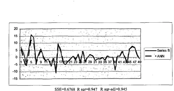
sqr-adj’ output, we can see that its value is 0.452 and it shows that this model can represent 45.2% of the time series or, in other words, it represents 45.2% better results than taking mean value of the series as a model. This can also be observed from the graphical output of the model in Figure 2. It is inferred from the values of the Ljung-Box statistics [ 9 ] that residuals of the model represent the process of white noise.

The results of the output obtained by Elman ANN structure are given in Figure 4 and Table 4. These are presented in the same format as the results from ARIMA model in series-graph and analytical data. From the output data the goodness of the fit can be determined. The value of

‘R

sqr-adj’ parameter is 0.945, and the sum of squared errors is 0.6768. It can be concluded that this model fits 94.5% to the process dynamics of the given time series. We have implemented only one AR parameter in this model. The fit goodness can by increased by increasing the number of the dependent variables up to 4 variables. However, when further increase of the number of dependent variables is employed the results are poorer, hence this does not contribute to significant improvement [SI. With two AR parameters, I % better results have been obtained than with one AR parameter. This is due to the recurrent mechanism of the ANN employed. Elman ANN takes into account previous values of the time series through the recurrent loops it possesses. Following the analyzed data and results, we can conclude that this time series could be

.-

.

- considerably better represented by a non-linear model

as compared to the linear case, Hence ANN-NARX is apparently advantageous.

Should now the values of Ljung-Box statistics on 5% level of significance are closely examined, it may well be noticed the residuals obtained via ANN-NARX modeling represent a stationary time series. Namely, values at lags 6, 24, 36, and 48 are above those in the Chi-square distribution.

Cr6 2

k,

Final Estimates of Parameters Type M A 1 M A 2 M A 3 M A 4 M A 5 SMA 6 Constant Coeff -0.0604 -0.0140 0.0187 0.0329 0.0603 0.9658 -0.03592 SECoeff T

P

0.0531 -1.14 0.257 0.0533 -0.26 0.792 0.0532 0.35 0.726 0.0532 0.62 0.537 0.0536 1.12 0.261 0.0192 50.34 0.000 0.01970 -1.82 0.069 Cr6 2luLModified Box-Pierce (Ljung-Box) Chi-

Square statistics

Lag 12 24 36 48

Chi-square 8.0 29.8 41.6 59.8

DF 5 17 29 41

P-Value 0.159 0,028 0.061 0.029 In this standard processing, the following data should be observed as well:

Differencing: regular, 1 seasonal of order 6 Number of observations: Original series 369,

Residuals:

SS

= 19125.4 (back-forecasts after differencing 362

excluded) M S = 53.9 D F = 3 S 5

Cr6 2ElModified Box-Pierce (Ljung-Box) Chi- Square statistics for Elman ANN modeling

Lag 6 12 24 36 48

Chi-Square 14.99 18.75 45.90 62.01 81.16 It is emphasized at this point that considerably better results have been obtained when processing all other cases of time series, including the ones for the specific applications in tourism and insurance business [SI.

Let now briefly discuss the results for the second case, U.S. HOG price data: annual, of well known time series.

Cr6

2k7.

Final Estimates of Parameters

Type Coeff SECoeff T P

MA 1 -0.1113 0.1066 -1.04 0.300 MA 2 0.1522 0.1087 1.40 0.165 MA 3 0.3774 0.1086 3.47 0.001

In

this standard processing, the following data should be observed as well:

0 Number ofobservations: 81,

0 _Residuals:

SS =

_{0.000315245 (back-forecasts} excluded) MS = 0.000004042 DF =78 Cr6

2H.

Modified Box-Pierce (Ljung-Box) Chi-

Square statistics

Lag I2 24 36 48

Chi-square 7.9 24.9 30.9 40.5

DF 9 21 33 45

P-Value 0.542 0.251 0.572 0.663 The

US.

HOG price data time series possesses a varying variance and therefore Box-Cox [9] transformation with k=-0.5 is applied first. Then, for the purpose of ARlMA modeling, one differencing is made to obtain its stationary equivalent, and according to Akaike [I], [2] and Bayesian Schwartz [3], [6],

[XI

criteria three MA parameters are used so that model AlUMA[O,1,3] is obtained. Results obtained are presented in Figure 5. The calculation of ‘R sqr-adj’ showed 0.186 or 18.6% better modeling representation than in the alternative when the average of the stationary equivalent was taken. Results

on

Ljung-Box statistics [9] at 5% level of significance have revealed that residual time series represent white noise process.

When this time series is modeled by means of Elman ANN-NARX the results shown in Figure 6 and Table 7 are obtained. As before, the original time series was processed by Box-Cox transformation and differenced ones, and thereafter normalized in the interval [-I, 11. For the modeling purpose one AR parameter and a constant has been used.

It

is noticed form both the graphical representation and the values

of

’R-sqr-aq’ that the output of the neural network emulates the evolution of the time series 97.4% better than in the alternative when the average of the stationary equivalent was taken. Results

on

Ljung-Box statistics at 5% level of significance have revealed that the residuals represent white noise process. Referring to Figure 5, one can easily that in this case time series the modeling representation by means of Elman ANN- NARX is almost ideal one.

Cr6 2lg. Modified Box-Pierce (Ljung-Box) Chi- Square statistics for Elman ANN modeling

Lag 12 24 36 4 8

Chi-square 9.475 9.515 9.581 9.726

IV.

CONCLUSION

A thorough investigation and comparison analysis on Box-Jenkins and Elman-ANN methodologies, also

involving the design and implementation of expert application-oriented software [SI, has been carried out with the prospect of their use in areas of insurance and tourism. These have been tested and verified by means of many time series and the two well known cases from literature [9] are used in this paper. Several different approaches can be applied to model economic processes and cycles in these areas, and both Box- Jenkins and Elman-ANN approaches can be successful. They are powerful tools for analysis that lead to deeper understanding of underlying evolution in recorded time series, hence better forecasting and control of the system dynamics. However, the two notoriously difticult case studies show that Elman-ANN approach offers superior toll in financial applications of insurance and tourism.

While neural networks implementing NARX model can fit a dataset much better than linear models, it has been found that under certain circumstances they may forecast poorly thus confirming previous observations. However, this does not happen when convergence rate rms bounds [IO] are satisfied. It is believed therefore that both these techniques for modeling and forecasting time series of economic nature and origin should be incorporated in a decision support system, and their respective potentials exploited in parallel. This research is in progress towards the third alternative modeling that uses fuzzy regression, and its comparison analysis with the ones explored insofar.

111 121 131 141 151 161 171 181 V. REFERENCES

H. Akaike, “ A new look at statistical model identification”. IEEE Trans. on Aulomatic Control,

vol. 19,pp. 716-723, 1974.

H. Akaike, “Canonical correlation analysis of time series and the sue of an information criterion”. In:

System Identijicorion: Adovancer and Care Studies, cd.

R.K. Mehra and D.G. Lainiotis.

New

York Academic Press, 1976, pp. 27-96.

T.W. Anderson, The Statistical Analysis of Time

Series.

New

York Wiley, 1971.

C.J. Andreeski, G.M. Dimirovski, “A memory NN- computing stmchm for identification of non-linear process dynamics”. In: Automatic Systems for Building

the lnfmmchrre in Devebping Counbies (Knowledge ond Technology Transfer), ed. G.M. Dimirovski. Oxford Pergamon Elsevier Science, 2001, pp. 3 9 4 . C.J. Andreeski, Analysis of Economic Time Series: Algorithms and Application Software for Model Dvelopement (ASE-ETF Techn. Report ETS-01/2001). Skopje: SS Cyril and Methodius University, 2001. R. Bastos, C. Predencio, T.

B.

Ludermir, Evolutionary design of”, Recife Brad; [rbcp, tbl]@cin.ufpe.br. G.E.P. Box, “Use and abuse of regression”.

Technometrics, vol. 8, pp. 625429, 1966.

G.E.P.

Box and G.M. Jenkins, Time Series Analysis:

Forecasting and Connol. San Francisco C A Holden- Day, 1970.

[9] G.E.P. Box, G.M. Jenkins, G. C. Reinsel, Timeseries

Analysis: Forecosring ond Control (3” ed.). Englewood Cliffs, NJ: Prentice Hall, 1994.

[ I O ] X. Cheng, I. Facine & N.R. Swanson, “Semiparametric ARX neural-network models with an application lo forecasting inflation”. IEEE Trans. on

NmrdNemorkr, &&Pc (4). pp. 674-683, July, 2001. [ I l l G. Doffner, Neural Networks for Time .Series

Pmcessing (” Group Publications). Vienna: University of Vienna and Austrian Research InStiNte for AI; http://wvw.ai.univie.ac.at/oefai/ nni nngroup. html#Publications.

[U] F.S. Hillier, G.J. Liebeman, Inrroduchon to

OperalionsResearch. New York Mc-Graw Hill, 1995.

[ 1 3 ] L. Ljung, T. S6dentr6m Theory and Prucrice of

Recusrive Idenhrficarion. Cambridge, MA: The MIT Press, 1983.

[I41 L. Ljung, System Idenrifcution: Theory for rhe User.

Englewood Clifss, NJ: Prentice-Hall, 1987.

[ISJ A.-M. S. Yaser, A.F. Atiya., M. Magdon-lsmail, H. white, “Introduction to the special issue on neural networks in financial engineering”. IEEE Trans. on

Nwrul Nemorkr, vol. 12, no. 4, pp. 653-656, July, 2001.

I

Fig. 2. Stationary data obtained from Series B IBM (original series taken from the literature) C r 6 2 t W u t p u t

from

BSC criteria 20 15 10 5 0 -5 -10 -15 l

20 15 10 5 0 -5 -10 -15 . . SSE=0.6768 R s q A . 9 4 7 R sqr-adj4.945

Fig. 4. Graph representation of series and analytical output of the modeling with ANN-NARX model for case

1

0,008 0.006 0.004 0.002 -Series 0 -0.002 -0,004 -0.006

Fig. 5 .

.

Graph representation of series and analytical output of the modeling with ARIMA model for case

2

0,008 0.006 ! 0,004 0.002 -Series 0 -0.002 -0.004 -0.006 SSE=0.1585 R s q r 4 . 9 8 0 R sqr-adj=0.974