SIHGIE MAGI I f E - S C l E D D l l i i G P E O M E MS :
Y - I A I B Y . P E I A I I I E S
A THESIS
SUBMITTED TO THE DEPARTMENT OF INDUSTRIAL ENGINEERING
AND THE INSTITUTS OF ENGINEERING AND SCIENCE
OF SiLKENT UNIVERSITY
m
PARTIAL FULFILLMENT OF THE REOUmEIVlENTS
FOR THE.DEGREE OF
DOCTOR Or PHILOSOPHY
s y■weyoa Oguz
I V i s a r i 'h I Q Q J ? d <S ii Uw(S i ’f S w j|.r ’^uaiSINGLE MACHINE SCHEDULING PROBLEMS:
EARLY-TARDY PENALTIES
A THESIS
SUBMITTED TO THE DEPARTMENT OF INDUSTRIAL ENGINEERING AND THE INSTITUTE OF ENGINEERING AND SCIENCE
OF BILKENT UNIVERSITY
IN PARTIAL FULFILLMENT OF THE REQUIREMENTS FOR THE DEGREE OF
DOCTOR OF PHILOSOPHY
By
Ceyda Oguz
March 1993
A S IS
.0 3 g Ï 0 3 3
C 'f ß i s a
I certify that I have read this thesis and that in my opinion it is fully adequate, in scope and in quality, as a dissertation for the degree of Doctor of Philosophy.
Assoc. Prof. Dr. Cemal Dinçer (Supervisor)
I certify that I have read this thesis and that in my opinion it is fully adequate, in scope and in quality, as a dissertation for the degree of Doctor of Philosophy.
Prof, alim Doğrusöz
I certify that I have read this thesis and that in my opinion it is fully adequate, in scope and in quality, as a dissertation for the degree of Doctor of Philosophy.
I certify that I have read this thesis and that in my opinion it is fully adequate, in scope and in quality, as a dissertation for the degree of Doctor of Philosophy.
C D
Assoc. Prof. Dr. Ömer Benli
I certify that I have read this thesis and that in my opinion it is fully adequate, in scope and in quality, as a dissertation for the degree of Doctor of Philosophy.
C\7^
Assoc. Prof. Dr. Suna Kondakçı
Approved for the Institute of Engineering and Science:
Prof. Dr. Mehmet Baidy,
Abstract
SINGLE M ACH INE SCHEDULING PROBLEMS:
E A R L Y -T A R D Y PENALTIES
Ceyda Oğuz
Ph. D. in Industrial Engineering
Supervisor: Assoc. Prof. Dr. Cemal Dinçer
March 1993
The primary concern of this dissertation is to analyze single machine total earli ness and tardiness scheduling problems with different due dates and to develop both a dynamic programming formulation for its exact solution and heuristic algorithms for its approximate solution within acceptable limits. The analyses of previous works on the single machine earliness and tardiness scheduling problems reveal that the research mainly focused on a restricted problem type in which no idle time insertion is allowed in the schedule. This study deals with the general case where idle time insertion is allowed whenever necessary. Even though this problem is known to be A'P-hard in the ordinary sense, there is still a need to develop an optimizing algorithm through dynamic programming formulation. Development of such an algorithm is necessary for further identifying an approximation scheme for the problem which is an untouched issue in the earliness and tardiness scheduling theory. Furthermore, the developed dynamic programming formulation is extended to an incomplete dynamic programming which forms the core of one of the heuristic procedure proposed.
A second aspect of this study is to investigate two special structures for the different due dates, namely Equal-Slack and Total-Work-Content rules, and to discuss computational complexity of the problem with these special structures. Consequently, solution procedures which bear on the characteristics of the special due date structures are proposed. This research shows that the total earliness and tardiness scheduling problem with Equal-Slack rule is A/’P-hard but can be solvable in polynomial time in certain cases. Moreover, a very efficient heuristic algorithm is proposed for the problem with the other due date structure and the results of this part leads to another heuristic algorithm for the general due date structure.
Finally, a lower bound procedure is presented which is motivated from the structure of the optimal solution of the problem. This lower bound is compared with another lower bound from the literature and it is shown that it performs well on randomly generated problems.
K e y w o rd s : Deterministic Single Machine Scheduling, Minimizing Total Earliness and Tardiness, Computational Complexity Theory, Dynamic Programming, Heuristic Algorithms, Lower Bounds.
özet
Т Е К M A K İN A ÇİZELGELEM E PROBLEMLERİ:
E R K E N -G E Ç PENALTILARI
Ceyda Oğuz
Endüstri Mühendisliği Doktora
Tez Yöneticisi: Doç. Dr. Cemal Dinçer
Mart 1993
Tek makinalı farklı teslim tarihli toplam erken-geç çizelgeleme problemlerini analiz etmek ve problemin hem kesin çözümü için bir dinamik programlama formülasyonu hem de yaklaşık çözümü için kabul edilebilir sınırlar içinde sezgisel yordamlar geliştirmek bu çalışmanın ana içeriğini oluşturmaktadır. Tek makinalı erken-geç çizelgeleme problemleri üzerine daha önce yapılmış çalışmaların incelenmesi, araştırmaların başlıca, çizelgede boş zaman ilave edilmesine izin verilmeyen, kısıtlı bir problem üzerine yoğunlaştığını göstermektedir. Bu çalışma, gerekli olduğu zamanlarda boş zaman ilavesine izin veren genel modelle ilgilenmektedir. Tek makinalı erken-geç çizelgeleme problemleri için, MV-zov olmalarına rağmen, dinamik programlama formülasyonu yoluyla eniyi çözüm veren algoritmalara ihtiyaç vardır. Böyle bir algoritma, problem için bir yaklaşık yöntem tanımlayabilmek için gereklidir ki bu erken-geç çizelgeleme kuramında hemen hiç dokunulmamış bir alandır. Bundan başka, geliştirilen dinamik pro gramlama formülasyonu, önerilen sezgisel yöntemlerden birinin özünü oluşturan kısıtlandırılmış durum uzaylı bir dinamik programlama şekline dönüştürülmüştür.
Bu çalışmanın ikinci bir safhası farklı teslim tarihleri için iki özel yapının, Eşit-Boşluk ve Toplam-Iş-Içeriği kurallarının, incelenmesi ve bu özel yapılarla problemin hesap karmaşıklığının tartışılmasıdır. Bu problemler için, özel teslim tarih yapılarının özelliklerine dayanan çözüm yöntemleri önerilmiştir. Eşit-Boşluk kurallı toplam erken-geç çizelgeleme probleminin M V-zor olduğu ispatlanırken, problemin belirli durumlarda polinom zamanda çözülebildiği de gösterilmiştir. Bundan başka, ikinci teslim tarihi yapısı ile problem için çok etkin bir sezgisel yordam önerilmiş ve bu problemden elde edilen sonuçlar, genel teslim tarihli problem için bir başka sezgisel yordamın geliştirilmesine öncülük etmiştir.
Son olarak, problemin eniyi çözümünün yapısından kaynaklanan bir alt sınır yöntemi sunulmuştur. Bu alt sınır, literatürden bir başka alt sınır ile kıyaslanmış ve geliştirilen bu alt sınırın rassal yaratılan problemler üzerinde iyi performans gösterdiği gözlemlenmiştir.
Anahtar
Sözcükler: Deterministik Tek Makina Çizelgelemesi, Toplam Erken-Geç Enazlanması, Hesap Karmaşıklığı Teorisi, Kesin Çözüm Al goritmaları, Dinamik Programlama, Sezgisel Yordamlar, Alt Sınırlar.
Acknowledgement
I would like to express my appreciation to all those who have contributed directly or indirectly to this dissertation. I am grateful to Assoc. Prof. Cemal Dinçer for his invaluable supervision and encouragement throughout the development of this thesis. I am indebted to him for his interest and belief in my work. Above all, I gained the experience of conducting independent research and I thank him for his contribution to that.
I debt special thanks to Prof. Halim Doğrusöz, Assoc. Prof. Mustafa Akgül, Assoc. Prof. Ömer Benli, Assoc. Prof. Suna Kondakçı for their valuable remarks and discussions on the subject.
I would like to thank Prof. Thomas L. Morin for his contribution to the incomplete
dynamic programming part of the thesis. His valuable discussions and comments
were particularly helpful and led my research in new directions. I would like to express my thanks to referees, who have provided valuable comments on the papers to be published from this dissertation, for investing their time carefully reading the papers.
I owe substantial thanks to Dr. Cemal Akyel who acquainted me with the fascinating world of scheduling theory. I much appreciate the discussions with him at the various stages of this study. His morale support and encouragement throughout this study is greatly acknowledged.
Last but not the least, my sincere thanks are due to my family for their continuous morale support.
Contents
Abstract i Özet iii Acknowledgement v Contents vi List of Figures x List of Tables xi 1 Introduction 11.1
Problem D e fin itio n ... 41.2
Classification of Machine Scheduling P rob lem s...8
1.3 Combinatorial O p tim ization ... 9
1.3.1 Computational Complexity...
10
1.3.2 O p tim iz a tio n ...
11
1.3.3 A p p ro x im a tio n ...
12
1.4 Outline of this T h esis... 13
2 Review of Single Machine Earliness and Tardiness Problems 15
2.1
Problem C h a ra cteristics... 162.2 Classification of Earliness and Tardiness P roblem s... 18
2.3 Mathematical Formulation of the Problem, l|dj| Y^{wj Ej + Vj Tj) 20 2.4 Special C a s e s ... 23 2.5 Well Solvable C a s e s ... 25 2.5.1 \\d\Z{wjEj + V j T j ) ... 25 2.5.1
.1
l\ d > P \ ^ {w E j + v T j ) ... 25 2.5.1.2 l\d\J2wj{Ej + T j ) ... 28 2.5.2 l\d > 5\Z{Ej + T j ) ... 30 2.5.3 l \ \ j :g j { E / T ) ... 32 2.6 A/’P-hard P ro b le m s ... 34 2.6.1 1 |d < <^| J2{wj Ej + V j T j ) ... 34 2.6.2 l \ d < S \ Z { E j i - T j ) ... 35 2.6.3 l\dj\J2{wj Ej + V j T j ) ... 36 2.6.4 l\dj\Z{Ej + T j ) ... 382.6.4
.1
Scheduling of a Fixed Job Ordering for l\dj\Y^{Ej + T , ) ... 392
.6
.4.2
Optimizing A lg o r ith m s ... 422.
6
.4.3 Heuristic Algorithm s... 463 Solution Procedures for \\dj\Y^[Ej -\-Tj) 52 3.1 A Dynamic Programming A lg o r it h m ... 54
3.2 An Incomplete Dynamic Programming A lg o rith m ... 58
3.3 A Heuristic A lg o r it h m ... 60
3.4 Computational E xperien ce... 63
3.5 Concluding R e m a r k s ... 71
4 + Tj) with Special Structures for Distinct Due Dates 73 4.1 Problem l|djl + Tj) with Equal-Slack R u le ... 75
4.1.1 Analysis of l\dj = pj -f q\ Y,{Ej T j ) ... 75
4.1.2 Analysis of l|aj = <j' > — aj|... 77
4.1.3 Analysis of l|aj = ^ < |S'j — O jl... 81
4.1.4 vVP-Hardness of l|aj = ^ < i?| |5j — aj\ 85 4.1.5 Concluding R e m a rk s ... 89
4.2 Problem l\dj\Y^{Ej + Tj) with Total-Work-Content R u l e ... 89
4.2.1 Analysis of l\dj = kpj\Y^{Ej + Tj) ... 90
4.2.2 A Heuristic Procedure for \\dj = kpj \ + ' ^ j ) ... 95
4.2.3 Computational Experience for l|dj = A: Pj I -f Tj) . . 96
4.2.4 Concluding R e m a rk s ... 98
5 Further Results for l|dj I X^(E'j-f Tj) 100
5.1 An Alternative Heuristic Algorithm for l|c?j| ^ { E j + Tj) ...101
5.2
A Lower Bound for \\dj \ Y^{Ej + T j ) ...1056 Conclusions and Future Research 111
List of Notations References V ita 116 120 127 IX
List of Figures
1.1 Data of each exam ple...
6
1.2
Schedule of a for the e x a m p le ...6
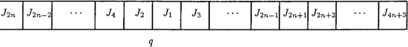
2.1 Job pair for the counter e x a m p l e ... 50
4.1 Schedule of a for Proposition 4.4... 78
4.2 Schedule of cr for Proposition 4.5... 79
4.3 Schedule for Proposition 4.9... 83
4.4 Schedule for Lemma 4.1... 87
4.5 The schedules a and cr'. 93 5.1 The schedules a and a'... 102
List of Tables
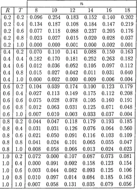
3.1 Average (AVG) and maximum (M AX) relative errors together with percentage of optimal solutions found by different rules for different
n values... 65
3.2
Frequency distribution of solution of different rules for n =8
andn = 10...
66
3.3 Frequency distribution of solution of different rules for n — 12 and n = 14... 67 3.4 Frequency distribution of solution of different rules for n = 16 and
n = 18... 67 3.5 Average relative errors of 5 problems for every pair of R and T
values for every n value for H E U R ...
68
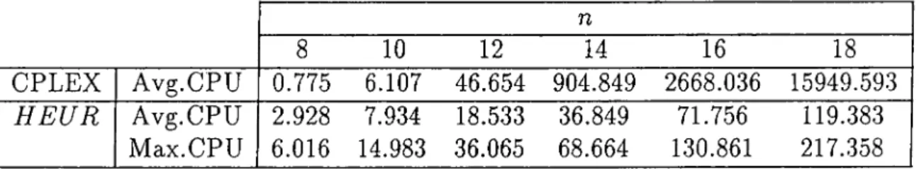
3.6 CPU times (in seconds) of the problems for different n values. . . 69 3.7 Computational Experience of Part II... 70 4.1 Average and maximum relative errors together with number of
optimal solutions found by different rules for different n values. . . 98 5.1 Average and maximum relative errors together with percentage of
optimal solutions found by different rules for different n values. . . 104
5.2 Average and maximum relative errors for LB and LBk y and number of problems LB > LBk y for diflFerent n values...110
Chapter 1
Introduction
Scheduling finds its application in a wide range of area whenever the problem of
“the allocation of resources over time to perform a collection of tasks” (Baker, 1974) arises. For example, it is possible to make an assignment of classes to the classrooms in academic institutions. As a classic problem, we may encounter with outpatient visits to doctors in the hospitals. Another example can be given from the computer systems as the processing of the independent jobs on the processors. In all these examples, the first items (classes, outpatient visits, independent jobs) are the collection of tasks and the second items (classrooms, doctors, processors) are the resources and we can extend these examples to encompass a larger variety of activities of everyday life.
We can easily argue that the tremendous research since the early 1950’s on the theory of scheduling is induced by this obvious practical importance and hence, it is not surprising that an impressive and enormous amount of literature has been evolving. But a careful investigation of the literature manifests that the main motivation and stimulation behind the existence of the scheduling theory as an important area in the operations research is its practical relevance to production planning and computer scheduling problems.
Chapter 1. Introduction
manufacturing systems so that each task, called job, requires at most one resource, called machine, at a time. The problem of concern is to schedule jobs on machines of limited capacity and availability which is called machine
scheduling problem. The result of solving this problem is a schedule which
specifies for each job when and by which machine it is to be processed. The aim is to find a schedule that optimizes some performance measures. The rich assortment of machine environments, job characteristics, and optimality criteria give rise to multitudinous machine scheduling problems. Over the spectrum of these scheduling problems, this thesis is concentrated on the area of deterministic
machine scheduling.
Although, the scheduling models addressed by researchers have become more and more complex in order to better reflect the real situations through the years, they still have certain restrictive assumptions. The crucial assumption that is common in these models is related with the optimality criteria to measure the quality of the feasible schedules. The vast majority of the literature on machine scheduling pertain to regular performance measures which are non-decreasing in each of the job completion times. However, this type of performance measures may not interpret the practice and there are many important occasions when non-regular performance measures apply. For example, if the aim is the conformance to the due dates of the jobs, then the common practice is to penalize only the jobs which are finished after their due dates, called tardy jobs, ignoring the consequences of the jobs that complete before their due dates, called early jobs. In order to reach an acceptable optimality criterion, one has to measure the quality of a schedule on a criterion that incorporates the penalties arise from both early and tardy jobs which leads to a non-regular performance measure.
An important drawback of considering scheduling problems with non-regular performance measures lies in the difficulty of finding an optimal solution. The difficulty arises because in some cases the insertion of idle time between jobs will be beneficial which enlarges the set of feasible schedules. Regarding these two classes of the performance measures, this thesis is restricted to non-regular
Chapter 1. Introduction
performance measures. Considering the hardness of these models, we further restrict ourselves to the single machine environments. Indeed, this last restriction is not so meaningless from both practical and theoretical point of view. First of all, because of its structural simplicity, it is easy to visualize the interactions in the model. It is also possible to explain the nature of the differences among different solutions and their relationships to different performance measures. Furthermore, the solutions of the single machine scheduling models can be used in more complex scheduling models by either being a basis for their solution procedures or supplying approximate but practical solutions. From a practical point of view, in addition to the existence of many shops which are actually a single machine, there are cases in which large and complex shops behave as if they are single machine environments. Examples of the latter can be seen in the chemical industries. Besides, there are many shops with more than one machine but either there is a single machine dominating all other machines in terms of job density or there exists a bottleneck machine, hence, viewing the shop as a single machine environment is an acceptable approximation.
More specifically, this thesis focuses on the deterministic single machine scheduling problems with the optimality criterion that aggregates the tardiness and earliness into a single objective function. In this introductory chapter, we present an overall view of single machine scheduling earliness and tardiness problem. We define the single machine earliness and tardiness problem formally in Section
1.1
and then elaborate on the reasons for involving both earliness and tardiness penalties in the objective function. In Section1
.2
, we give the notation used throughout this thesis to represent scheduling problems which is based on the classification of machine scheduling problems introduced by Lawlerei al. (1989). In Section 1.3, we point out how machine scheduling problems fit into the broader framework of combinatorial optimization and give an informal introduction to the theory of computational complexity. With the help of this theory, it is possible to classify problems as easy or probably hard to solve.those concepts that are relevant for the subsequent chapters are discussed; others are merely touched upon. For more elaborate introductions to the respective areas, we refer to Conway et al. (1967), Baker (1974), Lawler et al. (1989) for machine scheduling and to Garey and Johnson (1979) for computational complexity.
Chapter 1. Introduction
4
1.1
Problem Definition
In the single machine total earliness and tardiness problem, we are given a set
J = (J i, J
2
, · · ·) of n independent jobs to be processed on a single machine that can handle at most one job at a time without preemption. In an instance of this problem, a processing time pj G a ready time Vj G Z~^ on which jobJj becomes available for processing, a due date dj G Z ^ by which job Jj should
ideally be completed, and weights wj G Z~^ and Vj G Z^ indicating the relative importance of job Jy as being early and tardy, respectively, can be specified for each job Jp We can also determine for every job Jy a target starting time
ay
= dy — Pj by which jobJy
should ideally be started. Given a processing order on the single machine, the starting time 5y, the completion time Cy = Sj +py, the tardiness Ty = max{0,Cy — dy), the earliness Ej = max{0,dy — Cy} and the lateness Lj = Cy — dy for each jobJy
can be computed such that the capacity and availability constraints of the machine are not violated. In an instance of this problem, we will use <5 and C for the set of starting times and the set of completion times, respectively. The penalties will be given in the set V where, in this representation, the negative and the positive values denote the earliness and the tardiness of a jobJy,
respectively. The quality of a schedule is measured in terms of the optimality criterion which is the scheduling cost incurred as a function of the earliness and the tardiness of each jobJy,
stated as gj{E^ T). The optimality criteria covered in this study involve the minimization ofmaxi max Ei, max TA
or of
E f t
6
(E ( i ^ i + T ,),Y :(w iE j + VjTi)}where E ft' = J l]=iS i{E IT ) with g j(E IT ) = (£,■ + Tj), and (wjEj + VjTj), respectively.
In the analysis of the given scheduling problem, we will use the following additional notation:
•
7
T and cr denote sequences of jobs. Furthermore, and denote the set of jobs that form the sequences tt and cr, respectively.•
7
t(z) and cr(z) denote the z-th job in the sequence. Hence, i is the position index and i —1
,2
, . . . , n.• z{a) denotes the value of the optimality criterion for the schedule of cr and
unless otherwise stated.
• S {£s) represents the set of jobs that complete before the due date (target starting time), where \E\ (li’sl) denotes the cardinality of E (Es).
• E' (E^) represents the set of jobs that complete exactly on or before the due date (target starting time), where \E'\ denotes the cardinality of E' № )■
• T {Ts) represents the set of jobs that start exactly on or after the due date (target starting time), where |T| (IT^I) denotes the cardinality of T {Ts).
• T ' {Tg) represents the set of jobs that complete after the due date (target starting time), where \T'\ (I'T^j) denotes the cardinality of T ' {Tg).
Chapter 1. Introduction
5
We illustrate these notions by two 5-job examples for different due date structures. In the first example, all jobs have the same due date which is called as a common due date, d. In the second example, all jobs have a different due date but all have a common target starting time, q. The data are given in Figure
1
.1
. AnChapter 1. Introduction a) j 1 2 3 4 5 b) j 1 2 3 4 5 Pj 3 4 5 6 7 Pi 3 4 5 6 7 dj 17 17 17 17 17 di 18 19 20 21 22 a) h)
F igu re
1
.1
: Data of each example----i L E _____ ^ ---► -T Js Jl J2 J
4
14 17 21 27 Ja Jl J3 Js 11 15 18 2311
9 t 30F igu re
1
.2
: Schedule of cr for the examplearbitrary schedule of a is represented in the Gantt Chart in Figure
1.2
for each example.Scheduling problems consisting earliness and tardiness penalties in their objective function may have many applications in industry where both early and late completion of jobs from their due dates are costly and hence undesirable. For example, both earliness and tardiness penalties are in the nature of production environments such as having perishable products or applying Just-In-Time concept, since the deliveries should be coordinated with the manufacturing process steps due to the less adjustable delivery times than process steps.
Chapter 1. Introduction
The inclusion of an earliness cost in the objective function may represent the cost of completing a project early in PERT-CPM analyses, as suggested by Sidney (1977). Apart from these, we can give the example of scheduling a sequence of experiments that depend on predetermined external events such as the position of the sun as a natural application of earliness and tardiness penalties. If we consider the completion of a job after its due date, it is common to incur costs due to the loss of the order and loss of customer goodwill. The cost of tardiness also includes customer dissatisfaction, contract penalties and potential loss of reputation. On the other hand, completion before the due date may lead to higher inventory costs, increases the danger of over-stocking in the event of order cancellation, and if goods are perishable, causes potential loss of usable production due to their deterioration. If it is assumed that once a job completes its processing, it is free to leave the system, then earliness will not be a problem. But in many cases, customers do not want to receive orders early since they will hold unnecessary inventory. This can cause the cash commitment to resources in a time frame earlier than needed.
Indeed, earliness costs have a different nature from tardiness costs because they are of an indirect nature. Early jobs tie up capital, take up scarce floor space, and generally indicate that resource allocation and utilization may have been less than optimal. In essence, the cost of earliness is a cost of inefficiency and represents an unproductive investment which implicitly incurs an opportunity cost. Since minimizing the earliness and tardiness penalties has important practical applications, the research on scheduling problems with earliness and tardiness penalties are growing rapidly.
1.2
Classification of Machine Scheduling
Problems
Since there exists multifarious machine scheduling problems, we need a classification scheme to make them rapidly accessible and easy to refer to. We follow the notation and terminology of the classification scheme for deterministic machine scheduling problems as suggested by Lawler et al. (1989). In this notation each scheduling problem is represented by means of three parameters a, ^ ,
7
, where:Chapter 1. Introduction
8
• cc identifies the machine environment, such as single machine (
1
). We do not deliberate on the multi-machine environments, for which a has many different expressions, since our research deals with single machine environment.• /3 C { ^ i , . . . , / ?
4
} identifies the job characteristics, which are defined as follows:-
^1
e {p m in ,0
}.= pmtn\ Preemption is allowed: the processing of any operation may be interrupted and resumed at a later time.
/?i = 0: No preemption is allowed. -
^2
G0
}·= T'y Release dates that may differ per job
Jj
are specified./32 = 0: All r,· = 0.
~ ^3 € {pj =
1
,0
}.Ps = Pj = Each job Jj has a unit processing requirement.
^3
= 0: All Pj are arbitrary nonnegative integers. - ^4 G {d, dj, 0)./?4
= d: Acommon
due date is specified for each jobJj.
/?4
= 0: Due dates are variables, the values of which have to be determined.•
7
identifies the optimality criterion of the scheduling problem, such as the total unweighted earliness and tardiness penalties +Tj).
A three-field-notation scheme a\/3\'f will be used to describe a machine scheduling problem. Hence, the problem of determining an optimal single machine schedule with minimum total earliness and tardiness penalties is denoted by
\\dj\ Yigj{E /T), following the above terminology.
Chapter 1. Introduction
9
1.3
Combinatorial Optimization
Machine scheduling problems belong to the area of combinatorial optimization. Combinatorial optimization involves problems in which we have to choose the best from a finite number of relevant (feasible) solutions over a combinatorial
(discrete) set. For the total earliness and tardiness scheduling problems that are
of concern, for instance, we can restrict ourselves to the n! permutations of the
n jobs. Indeed, the solution space is larger than this, since for each permutation
(or sequence) there is more than one feasible schedule due to the inserted idle times before or between the execution of jobs. But the optimal schedule can be obtained easily once a sequence is specified (see Section 2.6.4).
The finiteness of the solution set by implying the effectiveness of the brute-force approach of explicit enumeration may be misleading. Since the optimal solution can be obtained by a straightforward method that generates all feasible solutions and select the best one with respect to its objective function. Unfortunately, however, the efficiency of this type of enumeration methods is far from being satisfactory for solving large scale problems of practical importance since the required effort to examine all schedules grows exponentially with the number of jobs.
Chapter 1. Introduction 10
We have therefore good reasons to search for faster algorithms. At this point a fundamental question is whether a problem is ‘well solved’ (‘easy’) or ‘hard’ . The distinction between easy and hard problems apparently involves the effort required to solve them to optimality. Since the effort grows with the size of the problem instance, it makes sense to express the effort as some function of this size. The size o f an instance is defined as the number of symbols required to represent an instance and this depends on encoding that is the representation system we employ. Integers may be represented by an arithmetic system to some fixed base jB >
2
, in which case [log^ n] symbols are required to represent an integer n. If jB = 2, then we have a binary encoding. Another system is a unaryencoding. Under a unary encoding, integers are represented by a series of I ’s, the length of which is equal to the value of the integer: to represent an integer n, we need n symbols.
The time complexity of an algorithm for a given problem is measured by an upper bound on the number of computation steps that the algorithm performs on any valid input, expressed as a function of the size of the input. If the size of the instance is measured by n, then the running time of an algorithm is expressed as O { f { n) ) if there are constants c and no such that the number of steps for any problem instance with n > no is bounded from above by c /( n ) , for some function / .
An optimization problem is said to be easy if there exists an algorithm that solves the problem in time poiynomiaily bounded in the input size. On the other hand, if any algorithm for the problem requires a complexity not bounded above by a polynomial in n, it is considered to be hard.
1.3.1
Computational Complexity
In discussing the complexity of a problem, it is sometimes more convenient to use the decision problem rather than the optimization problem. The decision variant of a scheduling problem is defined as the following question: given an instance
Chapter 1. Introduction 11
of the problem and a threshold value y, does there exist a schedule with value no more than y? All easy decision problems constitute the class V. This class is a subset of the class A fP , which, in the present context, contains all decision problems for which it is possible to check in polynomial time if the answer is ‘yes’ for a given schedule. A decision problem is said to be complete if it belongs to A iP and if every problem in AfP is polynomially reducible to it. A problem n is said to be polynomially reducible to a problem II' if and only if an arbitrary instance of II can be solved by solving a corresponding instance of II' that is constructed in time polynomially bounded in the size of II. The optimization variant of an A/^7^-complete problem is called AfP-hard; these problems are at least as hard as all problems in AiP.
Coming to the diiferent encoding schemes, the distinction between binary and unary encoding of the input is relevant for those problems that are A/”'P-complete under a binary encoding, but solvable in polynomial time under a unary encoding. An algorithm which is polynomial under a unary encoding, but not polynomial under a binary encoding, is called a pseudo-polynomial time algorithm. Problems that are A/P-complete under both encodings are called strongly AiP-complete. Problems are said to be ordinarily AfP-complete if they are A/’T’-complete under a binary encoding. For details concerning computational complexity, refer to Garey and Johnson (1979).
1.3.2
Optimization
Although optimization algorithms for hard combinatorial optimization algorithms are unavoidably enumerativo in nature, the aim is still to develop algorithms that perform satisfactorily well on the average for instances of reasonable size. Dynamic programming and branch-and-bound are two major enumerativo methods to solve hard combinatorial optimization problems.
Both dynamic programming and branch-and-bound aim at implicit enumeration of the solution space. For the application of dynamic programming, we need to
Chapter 1. Introduction
12
identify some underlying principle of optimality. Application of the optimality principle may require both time and space that is not bounded by a polynomial in the length of the input. Nonetheless, dynamic programming based pseudo polynomial algorithms may be very efficient.
Branch-and-bound algorithm mainly consists of a branching structure of the problem which generates feasible set of solutions for smaller subsets of the original set, and lower and upper bounding functions as well as a dominance relation that together constitute a bounding operation which is used to discard some subsets from further consideration. The performance of a branch-and bound algorithm is affected firstly by the strength of the lower bounds which restrict the growth of the feasible sets. Furthermore, the quality of the upper bounds, the dominance relations, and also the branching structure directly affect the efficiency of a branch-and-bound algorithm.
1.3.3
Approximation
It is obvious that an optimization algorithm for a hard combinatorial optimization problem will take exponential amount of time in the worst case. This leads to deal with a good approximate solution which can be obtained in a reasonable time and with less effort instead of finding an optimal solution. For this case, the main question is the trade-off between the quality of the approximate solution and the time spent to find it.
There are a number of popular techniques for designing approximation algorithms for the machine scheduling problems. For example applying dispatching rules which make use of priority functions that associate an urgency measure for each job is one of the simplest and widely used technique. The second class contains the approximation algorithms based upon the dynamic programming and rounding which is known as incomplete dynamic programming. The main idea is to consider a specific part of the state space instead of the entire state space. The last class of techniques that we point out contains the local-search algorithms.
Chapter 1. Introduction
13
These type of algorithms first generate an initial schedule and then adjust it somewhat in order to improve the objective function value. One of the most widely used procedure is to define for a given schedule of a a neighborhood Na
as the set of schedules that can be obtained from a by carrying out a prespecified
type of changing operations, such as adjacent pairwise interchange.
Globally, we can say that local-search algorithms are easy to develop and implement, and are known to produce excellent results.
1.4
Outline of this Thesis
The main aim of this thesis is to analyze the single machine total unweighted earliness and tardiness scheduling problems. Although there exists considerable research for the case where all the due dates are same, the literature is limited on the problems where all the jobs have distinct due dates. There is a lack of both optimizing and heuristic algorithms for total earliness and tardiness scheduling problems with distinct due dates. The purpose of this study is to develop computationally efficient optimizing algorithms and heuristic algorithms that solve the addressed problem effectively. Another purpose of this research is to investigate some special structures for the due dates and then either to show that the problem is A/^'P-hard or to provide polynomial algorithms for the problem.
This thesis is organized as follows. In Chapter 2, the characteristics of the total earliness and tardiness problems are analyzed and previous work on these problems are reviewed concentrating on the problem l\dj\Yj{Ej + Tj). The discussion on the approaches of the problem l\dj\J2{Ej+Tj) concludes that there is a lack of both an exact algorithm and a heuristic procedure which solve this problem efficiently and effectively. One of the main chapters. Chapter 3, presents a detailed development of a dynamic programming formulation for the problem
Chapter 1. Introduction
14
dynamic programming. This approach forms also the basis for the heuristic procedure developed and this heuristic procedure is given in Chapter 3, together with the computational results. Chapter 4 analyzes two special structures for the distinct due dates of the problem l\dj\Yi,{Ej + Tj). In this chapter, it is shown that there exists two cases for the first structure. Chapter 4 first presents the equivalence of one of the cases to a polynomially solvable problem and then proves that the other one is AfV-hard. Chapter 4 also investigates the effect of a second special structure for the due dates on the problem l\dj\Yi,{Ej + Tj). After providing some properties regarding to this special structure, Chapter 4 concludes with an efficient heuristic algorithm. The first part of Chapter 5 extends the results obtained in Section 4.2 and develops an alternative heuristic algorithm for problem \ \dj \ Yi{Ej + Tj). In the second part of Chapter 5, a lower
bound procedure for problem \\dj \ Y^{Ej -\-Tj) is presented and its effectiveness is
tested on randomly generated problems. In Chapter
6
, the significance and the importance of the results of this study and possible directions for future research are discussed.Chapter 2
Review of Single Machine
Earliness and Tardiness
Problems
The subject of this thesis is to analyze the single machine total unweighted earliness and tardiness problems with distinct due dates. In this chapter, some of the early work on single machine total earliness and tardiness problems that is relevant to this research are briefly reviewed and analyzed. In the last section, Section 2.6.4, the main problem that we deal with is reviewed in detail which shows the deficiencies of the approaches on this problem.
In the following section, the characteristics and the basic definitions in the single machine earliness and tardiness problems are presented. Then, in Section
2.2
a classification of the earliness and tardiness problems is given. After giving the mathematical formulation of the problem in its most general form in Section 2.3, two special cases are stated in Section 2.4. Then, the problems that are categorized according to the classification given in Section2.2
are reviewed considering their complexity results in Section 2.5 and Section 2.6.2.1
Problem Characteristics
The objective function of the scheduling problems can be analyzed in two different classes. The first class consists of the one dimensional performance measures which are called regular performance measures. The second class is called as the
non-regular performance measures. A schedule for the sequence a is defined as a
vector of job completion times [(7i, (
72
, , (7„j. Then the performance measure can be denoted as:z{a ) = z {C ^ ,C ,,...,C n )
D efin ition
2.1
[Baker, 1974] A performance measure z{cr) is regular if(a) the scheduling objective is to minimize z[a), and
(b) z(a ) is non-decreasing in each o f the completion times, Cj, in the schedule.
This definition is important because it is usually desirable to restrict attention to a limited set of schedules called a dominant set. For example, in the single machine scheduling problem, the set of permutation schedules is a dominant set for any regular performance measures. That is, preemption and inserted idle time will never lead to a better schedule than the best permutation schedule for any regular performance measure.
Most popular performance measures, such as mean flowtime, mean lateness, mean tardiness, and number of tardy jobs, are all regular performance measures. There are, however, many applications in which non-regular performance measures are more appropriate.
D efin ition
2.2
A performance measure z{a ) is non-regular if the property (b)does not hold in Definition 2.1.
Chapter 2. Review o f Single Machine Earliness and Tardiness Problems
16
For example, the mean tardiness criterion has been a standard way of measuring conformance to due dates, although it ignores consequences of jobs completing
early. Hence, if it is desirable to meet all due dates exactly, it is necessary to consider non-regular performance measures. In spite of the importance of non-regular performance measures, very little analytical work has been done in this area probably due to the difficulty of solving these type of problems. The difficulty arises because in some cases the insertion of idle time between jobs will be beneficial which may prevent the set of permutation or non-delay schedules to be a dominant set. In this case, delay schedules should be considered which increase the solution space due to the inserted idle time in the optimal solution.
D efin ition 2.3 [Fry, Armstrong and Blackstone, 1987] A delay schedule is
any schedule where the machine is intentionally held idle when it could begin processing a job.
Theoretically, there are infinite number of delay schedules because arbitrary amounts of idle time can be inserted. However, this is not useful for a given sequence and a non-regular performance measure and we should restrict the feasible solution set to a finite number of schedules.
D efin ition 2.4 A local shift is changing the completion time o f a job in a feasible
schedule while keeping feasibility without changing the sequence.
D efin ition 2.5 [Davis and Kanet, 1992] A semi-active schedule for a non-regular
performance measure is one in which no local shift o f a job will provide a schedule with an improved value o f objective function.
Chapter 2. Review o f Single Machine Earliness and Tardiness Problems
17
It is obvious from the above definition that semi-active schedules dominate the set of all schedules. Since it is possible to insert some idle time between the jobs in a schedule, we can talk about a group of jobs such that there exists some idle time before the first job and after the last job of the group, but not between any two of the jobs in this group. We can state this concept formally as follows:
D efin ition
2.6
The blocks of the schedule are the maximal sets of jobsJjo, ■ ■ ·, Jji that are scheduled without any idle time between any two of these jobs, i.e., Sj-\-pj = V jo < j < ji, Sj^_i + P j,-i < (or jo = 1), and Sj^ + pj, < ¿jj+ i (or ji = n, the last position to be considered).
2.2
Classification of Earliness and Tardiness
Problems
Diversity in the total earliness and tardiness literature stem from the generality of assumptions made about the due dates and the optimality criteria. The single machine total earliness and tardiness problems can be classified according to
Chapter 2. Review o f Single Machine Earliness and Tardiness Problems
18
A. the condition on the due date:
1
. problems having a fixed common due date d for all jobs Jj y = i ,2
. . . . , n ) m ^ s A E I T ) )2
. problems having an individual due date dj for each Jj {j =1
,2
, . . . , n)m \ E s i ( E / T ) )
3. problems having the common due date d as a variable for all Jj
[j =
1
,2
, . . . ,n) (optimal due date assignment) (1
|| Y fgj[E ¡T ))B. its criterion that has usually been the minimization of total penalty cost as objective function, where the penalties can be measured in different ways:
1
. total unweighted earliness and tardiness (sum of absolute deviations of the job completion times from due date) {gj^E/T) = [Ej + Tj))2
. total weighted earliness and tardiness (weighted sum of absolute deviations of the job completion times from due date)Chapter 2. Review o f Single Machine Earliness and Tardiness Problems
19
Apart from these classifications, it is possible to talk about the objective function which is a function of the squared earliness and tardiness penalties. Such a problem, l|d| Yl,{Ej+T^), has been studied by Bagchi, Sullivan and Chang (1987). They define this problem as unrestricted if an increase in the due date does not result in any further decrease in the objective function value. That is, the due date does not constrain the minimization of mean squared deviation in any way. They have presented a general purpose branching procedure to solve this problem. Later, De et al. (1989) have demonstrated that for the restricted version of this problem, the branching procedure proposed by Bagchi, Sullivan and Chang (1987) does not always produce the optimal schedule. They have suggested an alternative approach that ensures optimality under all circumstances. They have also analyzed the derivation of bounds which are very useful in determining whether the problem is restricted or unrestricted. Furthermore, they have presented a solution procedure for the restricted problem.
Another criterion that has been studied in the literature is the minimization of maximum penalty of earliness and tardiness with different due dates. Sidney (1977) has considered this problem with penalties that are monotonically nondecreasing continuous functions of earliness (measured, in this case, as the deviation of the starting time from a given target starting time) and tardiness. Under restrictive assumptions on the starting times and the due dates, an
Ö (n^) algorithm for minimizing the maximum penalty has been presented in
the paper. For the same problem an О (n log n) algorithm has been later given by Lakshminarayan et al. (1978).
Baker and Scudder (1990) review the literature on the total earliness and tardiness scheduling problems providing a framework to show how results have been generalized starting with a basic model of a single machine common due date total unweighted earliness and tardiness problem. They also investigate more general models which are obtained by adding some features to the basic model such as parallel machines, complex optimality criteria and distinct due dates. Apart from this review, there has been a number of review studies about total
Chapter 2. Review o f Single Machine Earliness and Tardiness Problems
20
earliness and tardiness problems with different emphases.
Sen and Gupta (1984) survey scheduling models involving due dates. After classifying the scheduling problems according to their optimality criteria, they provide the theoretical developments and computational experiences within each category. The optimality criteria considered in this review include the minimization of a criterion related to the flow time of jobs, the set-up cost of machines, a criterion related to job lateness or tardiness, in-process inventories, and a combination of two or more of the above criteria.
Cheng and Gupta (1989) survey models in which the due dates are decision variables for both static and dynamic job shop situations. They analyze the static job shop for the case where the due date is constrained to be greater than or equal to the total processing times. For these type problems, the optimal due date and the optimal sequence are to be determined when the method of assigning due dates is specified. They discuss the identification of the most desirable due date assignment method for the dynamic job shops together with the literature dealing with determination of optimal due dates.
2.3
Mathematical Formulation of the
Problem,
l\dj\ E { w j E j+
Vj T j )This problem is the most general form of the total earliness and tardiness problems since it includes distinct due dates and weights for every job. This problem can be reduced to all other problems by defining the due dates and the weights appropriately.
Chapter 2. Review of Single Machine Earliness and Tardiness Problems
21
NLTETP: s.t. Min Y ,{w jE j + VjTj) j=i j=i j=l + Ej — Tj = dj Vi (2
.1
) 71 i=i >0
Wi (2
.2
) 71 =1
Vi (2.3) 711=1
=1
V; (2.4) Xij G {0
,1
} V i,i (2.5) C j, E j, Tj >0
Vi (2
.6
)where Xij is defined as
Xij 1 if
Jj
is assigned to position i0
otherwiseIn this model, the objective function is to minimize the weighted total earliness and tardiness of all jobs. Constraint
2.1
describes the earliness or tardiness of each job. From this constraint a job can only be either early or tardy, if it is not an on-time job. Constraint 2.2 prevents jobs to be overlapped. While constraint 2.3 denotes that exactly one job can be processed at every position, constraint 2.4 denotes that each job can be processed exactly at one position, that is no preemption is allowed. It can be seen that the model is nonlinear due to the constraint 2.2. Due to this nonlinearity, the computational difficulty of total earliness and tardiness problems increases. Fry, Leong and Rakes (1987) haveprovided another formulation for l\dj\Y^{wj Ej + V jT j) problem. Since, their formulation does not contain any nonlinearities, it is easier to handle. Their model, called MITETP, is provided below:
Chapter 2. Review o f Single Machine Earliness and Tardiness Problems
22
M ITETP:
Min 5^(u;,· Ei + Vi Ti)
i-l
s.t. k = l A;=l j = l n — dj Xij J=1 Vi (2.7)1
Vi (2
.8
) n t=l =1
Vi (2.9) X{j G {0
,1
} V i,i (2
.10
) Ei,Ti,Yi >0
Vi (2
.11
)where denotes the idle time to be inserted before the job at the ¿-th position. Hence, constraint 2.7 describes both the position of a job in the schedule, and its condition, that is being early, tardy, or on-time. Constraints 2.8, 2.9 and 2.10 are same as constraints 2.3, 2.4 and 2.5, respectively.
These models are important because the mathematical formulation of the problems is used in finding the optimal solution in our study. Hence, computationally tractable and efficient models are essential. Although the later model is a mixed-integer formulation and it is not efficient for large n values, it is notable in the sense that it overcomes the difficulties regarding the non-linear constraints of the former model. Furthermore, the former model is important because this type of formulation can easily be used in finding the optimal schedule
Chapter 2. Review o f Single Machine Earliness and Tardiness Problems
23
when a sequence is given. Because, once a sequence is determined, we can eliminate all the decision variables of Xij. In other words, since the technical constraints (or the precedence relationships) are all given, the NLTETP model turns out to be a linear programming model. In a formal way, we can state the linear programming model as follows:
LPTETP(<t): t=l s.t. “l·
^<^(0
— 4 (.) Vi (2
.12
) >0
Wi (2.13) >0
Vi (2.14)Note that, Cc{i) denotes the completion time where Ct^^o) — 0 a,nd pcr(i) denotes the processing time of the z-th job in the sequence cr, respectively. In this case, since a sequence is given, disjunctive constraints 2.3 and 2.4 of the NLTETP model are not necessary in LPTETP model. In this linear programming formulation, we have 3n variables and
2
n constraints. Although this model can be solved easily, there exists more efficient algorithms in the literature for finding the optimal schedule when a sequence is given (see Section 2.6.4).2.4
Special Cases
In this section, we present some more definitions which are used throughout the rest of this study. Some of these definitions are also required for stating the special cases for the problem.
D efin ition 2.7 In a Weighted Shortest Processing Time (WSPT) sequence jobs
are ordered according to non-decreasing ratios of processing times to the weight o f tardiness, i.e.,
P i/ v i< P2IV2 < . . . < Pnhn·
This sequence is called as Shortest Processing Time (SPT) sequence if the weight o f tardiness is equal to one for all jobs, that is if:
Vj = 1 V i = 1,2,
D efin ition
2.8
In a Weighted Longest Processing Time (W LPT) sequence jobsare ordered according to non-increasing ratios of processing times to the weight o f earliness, i.e.,
Pi/wi > P2IW2 > . . . > PnlWj,.
This sequence is called as Longest Processing Time (LPT) sequence if the weight o f earliness is equal to one fo r all jobs, that is if:
Wj = 1 V i = 1 , 2 , . . . ,n.
For total earliness and tardiness problems there exist two special cases which are true for all objective functions and restrictions about due dates (Ow and Morton, 1989).
1
. If WSPT sequence results in a schedule with no early jobs, then this is optimal schedule.2. If W LPT sequence results in a schedule with no tardy jobs, then this is optimal schedule.
Chapter 2. Review o f Single Machine Earliness and Tardiness Problems
24
Apart from these special cases, since the due dates are involved in the optimality criterion of the earliness and tardiness scheduling problems, it seems natural to have some sequencing rules that incorporates the information of due dates. One of such sequencing rules is the following:
D efin ition 2.9 In an Earliest Due Date (EDD) sequence jobs are ordered
according to non-decreasing values o f the due dates, i.e., d\ ^
¿2
^ · · · ^ ^n·A second sequencing rule that uses due date information is to consider target starting times (or equivalently the slack times) of the jobs as follows:
D efin ition
2.10
In an Earliest Starting Time (EST) sequence jobs are orderedaccording to non-decreasing values o f the target starting times, i.e.,
«1
<«2
< . . . < Un.Informally, the slack time of a job is the amount of time remaining before this job must be started if it is to be completed on time. This quantity is important because it shows the urgency of the jobs: smaller the slack time of a job, higher the chance of being tardy for that job.
2.5
W ell Solvable Cases
2
.
5.1 lldlEiwjEj + VjTj)
This problem is considered for two special cases according to the different weight assignments. In the first one all early jobs have the same weight w and all tardy jobs have the same weight v. In the second case, each job Jj has a weight luj which is independent of whether the job is early or tardy.
Chapter 2. Review o f Single Machine Earliness and Tardiness Problems 25
2.5.1.1 l\ d > P \ J 2 {w E j-i-v T j)
The problem l|d| Elj + vT j) is referred as the weighted sum o f absolute
firstly by Bagchi, Chang and Sullivan (1987). The problem l|d > +
v T j) is called as the unrestricted version of l\d\J2{'^ Ej + vT j) problem since
the due date is loose. The other case in which due date is tight is called as the restricted version. This distinction is important because while the unrestricted version can be solved in polynomial time, the restricted version has been shown to be j\7P-hard. To be more precise, l\d\'^(Ej + Tj) problem is defined as unrestricted ii d > P and restricted ii d < P, where P is the total processing time of the jobs in a schedule, i.e.,
n
p
=
Eft-The difference between two problems can be described qualitatively and in a simplified form. When the problem is unrestricted, since the due date is loose, there is more flexibility to construct the schedule such that d is in the middle of the schedule. In the restricted problem, however, this may not be possible since no job can start before time zero.
Bagchi, Chang and Sullivan (1987) have stated some propositions for the unrestricted version of the problem. These propositions restrict the search for an optimal solution to a limited set of schedules.
P ro p o s itio n 2.1 There is no inserted idle time between any jobs in the optimal
schedule (If job Jj immediately follows job Jk in the schedule, then Cj = Ckd-pj)· Chapter 2. Review o f Single Machine Earliness and Tardiness Problems
26
P r o o f: Assume the contrary. It is easy to see that the value of the objective function can be improved by eliminating the idle time between jobs. ■
D efin ition
2.11
A schedule is called V-shaped if the jobs completed on or beforethe common due date are in the W LPT order and the jobs completed after the common due date are in the WSPT order.
P r o o f: The proof follows from a simple job-interchange argument. ■
P r o p o s itio n 2.3 One job completes precisely at the common due date
(Cj
— d fo r some job Jj).P r o o f: The proof follows from a shifting argument of the schedule. ■
P ro p o s itio n 2.4 For d < Pi, the WSPT sequence is optimal. Furthermore, if
w < V, then the W SPT sequence is optimal for d < (pi p2)/2.
P r o o f: For d < pi, Proposition 2.4 is a well-known result. For w < v and
d < (pi + P
2
) /2
, the proposition can be established by job-interchange argument.Chapter 2. Review o f Single Machine Earliness and Tardiness Problems
27
P ro p o s itio n 2.5 In an optimal schedule the longest job is processed first.
P r o o f: Consider a schedule of a that satisfies Proposition 2.2 but violates Proposition 2.5. In such a schedule the longest job must be the last job in sequence. It is easily shown that the interchange of the first and the last jobs in
a improves the schedule. ■
P ro p o s itio n
2.6
For an optimal schedule o f the form {£ '){T ) one can write\n{vlvf\ for n{vIv) non-integer
where u — w + v.
n{v/u) or n(v/i/)-j-l fo r n iy ju ) integer
P r o o f: Similar to the proof of Proposition 2.7 in Section
2
.5
.2
. ■ For this problem an O (nlogn) algorithm is offered by Bagchi, Chang and Sullivan (1987) which is an alternative algorithm to the one given by PanwalkarChapter 2. Review o f Single Machine Earliness and Tardiness Problems
28
sequence with, optimal due date equal to d* where d* is the minimum due date for the optimal objective function. Jobs are scheduled by the algorithm one at a time, starting with the largest job and ending with the shortest job.
Panwalkar et al. (1982) have considered the problem of finding the best common due date for all jobs to minimize the total penalty which is the summation of weighted earliness and tardiness cost together with the due date assignment cost. A two-phased algorithm is given for solving this problem. In the first phase, the number of tardy jobs is found. Positional penalties, the optimal sequence and the optimal due date are found in the second phase. The algorithm subsumes the algorithm given by Kanet (1981) for minimizing sum of absolute deviation of completion times about a common due date as a special case.
2
.5 .1.2
l\d\^W j{Ej + Tj)Hall and Posner (1991) have shown that Propositions 2.1, 2.2 and 2.3 hold for the problem l\d\J2''^j + Tj) and presented four special cases for which the problem l\d\'^Wj{Ej -H Tj) is polynomially solvable. Hoogeveen and van de Velde (1992) has given one more special case for the problem l|(i| Wj (Ej J- Tj)
which is polynomially solvable:
W eig h ts and P ro ce ssin g T im es are Equal In this special case, = Pji j = 1 , 2 , . . . ,n. The algorithm proposed for this problem by Hall
and Posner (1991) is in O (n) and takes jobs in non-increasing order of their processing times and schedules them to finish early, until the total processing time of jobs scheduled is at least half of the overall total processing time. All other jobs are scheduled late. Since Wjlpj =