SOLUTION OF ELECTROMAGNETIC
SCATTERING PROBLEMS WITH THE
LOCALLY CORRECTED NYSTR ¨
OM
METHOD
a thesis
submitted to the department of electrical and
electronics engineering
and the institute of engineering and science
of bilkent university
in partial fulfillment of the requirements
for the degree of
master of science
By
Se¸cil Kılın¸c
September 2010
I certify that I have read this thesis and that in my opinion it is fully adequate, in scope and in quality, as a thesis for the degree of Master of Science.
Prof. Dr. Levent G¨urel (Supervisor)
I certify that I have read this thesis and that in my opinion it is fully adequate, in scope and in quality, as a thesis for the degree of Master of Science.
Prof. Dr. Ayhan Altınta¸s
I certify that I have read this thesis and that in my opinion it is fully adequate, in scope and in quality, as a thesis for the degree of Master of Science.
Assoc. Prof. ¨Ozlem Aydın C¸ ivi
Approved for the Institute of Engineering and Sciences:
Prof. Dr. Levent Onural
ABSTRACT
SOLUTION OF ELECTROMAGNETIC
SCATTERING PROBLEMS WITH THE
LOCALLY CORRECTED NYSTR ¨
OM
METHOD
Se¸cil Kılın¸c
M.S. in Electrical and Electronics Engineering
Supervisor: Prof. Dr. Levent G¨
urel
September 2010
The locally corrected Nystr¨om (LCN) method is used to solve integral equations with high accuracy and efficiency. Unlike commonly used methods, the LCN method employs high-order basis functions on high-order surfaces. Hence, the number of unknowns in the electromagnetic problem decreases substantially, this also reduces the total solution time of the problem. In this thesis, electromagnetic scattering problems for arbitrary, three-dimensional, and conducting geometries are solved with the LCN method. Both the electric-field integral equation (EFIE) and the magnetic-field integral equation (MFIE) are implemented. The solution time for Duffy integrals is reduced significantly by modifying the Duffy transform. Then, mixed-order basis functions are implemented to accurately represent the charge density for EFIE. Finally, both the accuracy and the efficiency (in terms of solutions times and the number of unknowns) of the LCN method are com-pared with the method of moments and the multilevel fast multipole algorithm.
Keywords: The locally corrected Nystr¨om (LCN) method, electromagnetic scat-tering, surface integral equations, high-order geometry modeling, high-order basis functions, the Duffy transform, radar cross section.
¨
OZET
ELEKTROMANYET˙IK SAC
¸ ILIM PROBLEMLER˙IN˙IN LOKAL
OLARAK D ¨
UZELT˙ILM˙IS
¸ NYSTR ¨
OM Y ¨
ONTEM˙IYLE
C
¸ ¨
OZ ¨
UM ¨
U
Se¸cil Kılın¸c
Elektrik ve Elektronik M¨
uhendisli˘
gi B¨
ol¨
um¨
u Y¨
uksek Lisans
Tez Y¨
oneticisi: Prof. Dr. Levent G¨
urel
Eyl¨
ul 2010
Lokal olarak d¨uzeltilmi¸s Nystr¨om (LDN) y¨ontemi, integral denklemlerinin y¨uksek do˘grulukta ve verimlilikte ¸c¨oz¨umleri i¸cin kullanılan bir metottur. Bu y¨ontemde d¨uzlemsel ¨u¸cgenler yerine, y¨uksek dereceli y¨uzeyler ¨uzerinde, y¨uksek dereceli temel fonksiyonları kullanılır. Bu sayede, elektromanyetik prob-lemdeki bilinmeyen sayısı azalmakta ve b¨oylece problemin ¸c¨oz¨um s¨uresi ¨onemli ¨
ol¸c¨ude kısalmaktadır. Bu tezde, ¨u¸c boyutlu, karma¸sık, m¨ukemmel iletken cisimler i¸ceren sa¸cılım problemlerinin LDN y¨ontemi ile y¨uksek do˘grulukta ¸c¨oz¨umleri ger¸cekle¸stirilmi¸s ve ¸c¨oz¨um s¨ureleri ile bilinmeyen sayıları momentler metodu ve ¸cok seviyeli hızlı ¸cokkutup y¨onteminden elde edilen sonu¸clar ile kar¸sıla¸stırılmı¸stır. LDN y¨ontemi hem elektrik-alan integral denklemi (EA˙ID), hem de manyetik-alan integral denklemine (MA˙ID) uygulanmı¸stır. Duffy d¨on¨u¸s¨um¨unde bazı de˘gi¸siklikler yapılarak toplam ¸c¨oz¨um zamanında b¨uy¨uk ¨ol¸c¨ude azalma sa˘glanmı¸stır. Ayrıca, tam dereceli temel fonksiyonları yerine karı¸sık dereceli temel fonksiyonları kullanılarak EA˙ID’de y¨uk¨un do˘gru modellenmesi sa˘glanmı¸stır.
Anahtar kelimeler: Lokal olarak d¨uzeltilmi¸s Nystr¨om (LDN) y¨ontemi, elektro-manyetik sa¸cılım, y¨uzey integral denklemleri, y¨uksek dereceli geometri mod-elleme, y¨uksek dereceli temel fonksiyonları, Duffy d¨on¨u¸s¨um¨u, radar kesit alanı.
ACKNOWLEDGMENTS
I would like to express my deepest gratitude to my supervisor Prof. Levent G¨urel, for his supervision, suggestions, and encouragement throughout the development of this thesis.
I would to like to thank to Prof. Ayhan Altınta¸s and Assoc. Prof. ¨Ozlem Aydın C¸ ivi for participating in my thesis committee and for accepting to read and review this thesis.
I am also thankful to the former and current researchers of the Bilkent Univer-sity Computational Electromagnetics Research Center (BiLCEM), especially to
¨
Ozg¨ur Salih Erg¨ul, for their cooperation and accompaniment in my studies. I would not be able to conduct high-quality research without their contributions.
My special thanks go to each member of my family for their endless love and patience.
Last but not least, thanks to Burak Tiryaki for being in my life, for witnessing every moment of this process, and for motivating me all the time.
◦
This work was supported by the Scientific and Technical Research Council of Turkey (TUBITAK) through a M.S. scholarship.
Contents
1 Introduction 1
1.1 Historical Background . . . 2
1.2 The Objective and Overview of the Thesis . . . 4
2 The Locally Corrected Nystr¨om Method 5 2.1 The Classical Nystr¨om Method . . . 6
2.2 The Locally Corrected Nystr¨om Method . . . 7
2.3 High-Order Geometry Modelling . . . 8
3 Application of the Locally Corrected Nystr¨om Method to the Electric-Field Integral Equation 12 3.1 Formulation . . . 13
3.1.1 Discretization . . . 16
3.2 Local Corrections . . . 17
3.2.1 Local Corrections for Self Patch . . . 19
4 Application of the Locally Corrected Nystr¨om Method to the
Magnetic-Field Integral Equation 25
4.1 Formulation . . . 26
4.1.1 Principal and Limit Value Integrals . . . 27
4.1.2 Discretization . . . 30
4.2 Local Corrections . . . 31
4.2.1 Local Corrections for Self Patch . . . 32
4.2.2 Local Corrections for Near Patches . . . 33
4.3 Excitation . . . 34
4.4 RCS Calculations . . . 35
5 Numerical Evaluation of the Integrals 36 5.1 The Duffy Transform . . . 37
5.1.1 The Duffy Transform for EFIE . . . 39
5.1.2 The Duffy Transform for MFIE . . . 39
5.1.3 Contribution to the Duffy Transform . . . 40
5.2 Adaptive Integration . . . 47
5.2.1 Method 1 . . . 48
5.2.2 Method 2 . . . 49
6.1 Discretization with the Mixed-Order Basis Functions . . . 53 6.2 Validation . . . 54
7 The Locally Corrected Nystr¨om Method Implementations 57
7.1 Current Results for Some Geometries . . . 58
7.2 RCS Results for Several Geometries . . . 58 7.3 Efficiency and Accuracy Comparisons with the MLFMA . . . 84
8 Conclusion and Future Work 89
Bibliography 90
9 Appendix A: Legendre Polynomials 95
9.1 Shifted Legendre Polynomials . . . 96
List of Figures
1.1 Solution of an electromagnetic scattering problem. . . 2
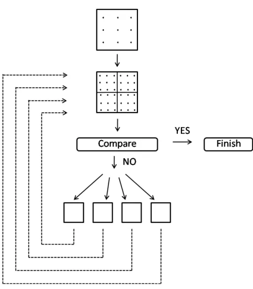
2.1 Discretization of various geometries with quadratic meshes: (a) square patch, (b) finite array of strips, (c) cube, (d) sphere, (e) NASA almond, and (f) ogive. . . 10 2.2 Nystr¨om discretization of various geometries: (a) square patch,
(b) finite array of strips, (c) cube, (d) sphere, (e) NASA almond, and (f) ogive. . . 11
3.1 Contour integral on unitary space required for the local corrections. 23
4.1 Observation point approaching to surface in the limit case. . . 28
5.1 (a) Singular point on the patch in the parametric space, (b) tri-angulated patch with common vertex at the singular point, and (c) mapping the Duffy-triangle into the unitary space. . . 38
5.2 The integrand plotted on the first triangle by using: (a) classical Duffy and (b) modified Duffy. . . 41 5.3 The integrand plotted on the second triangle by using: (a) classical
5.4 The integrand plotted on the third triangle by using: (a) classical Duffy and (b) modified Duffy. . . 43 5.5 The integrand plotted on the fourth triangle by using: (a) classical
Duffy and (b) modified Duffy. . . 44 5.6 Division of the quadrilateral region into triangular domains for the
(a) classical Duffy and (b) modified Duffy. . . 46
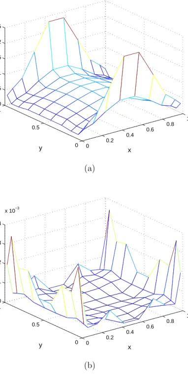
5.7 Relative error of classical and modified Duffy transforms for a
1λ× 1λ patch using the EFIE formulation. . . 47
5.8 Adaptive integration method 1. . . 48
5.9 Adaptive integration method 2. . . 50
6.1 (a) x component and (b) y component of the surface current den-sity on a 1λ× 1λ plate by using a 10 × 10 quadrature rule. . . 55 6.2 (a) x component and (b) y component of the surface current
den-sity on a 1λ× 1λ plate by using a 10 × 11 quadrature rule. . . 56
7.1 (a) x component and (b) y component of the surface current den-sity on a 1λ× 1λ plate, which is divided into four pieces, by using
a 5× 6 quadrature rule on each of the patches. . . 59
7.2 Current density results obtained with the LCN-EFIE formulation, (a) the geometry to be solved, (b) x component on the first patch, (c) x component on the second patch, (d) y component on the first patch, and (e) y component on the second patch. . . . 60
7.3 Current density results obtained with the LCN-EFIE formulation, (a) the geometry to be solved, (b) x component on the first patch, (c) x component on the second patch, (d) y component on the first patch, and (e) y component on the second patch. . . . 61
7.4 Current density results obtained with the LCN-EFIE formulation, (a) the geometry to be solved, (b) x component on the first patch, (c) x component on the second patch, (d) y component on the first patch, and (e) y component on the second patch. . . . 62 7.5 Current density results obtained with the LCN-EFIE formulation,
(a) the geometry to be solved, (b) x component on the first patch, (c) x component on the second patch, (d) y component on the first patch, and (e) y component on the second patch. . . . 63
7.6 Current density results obtained with the LCN-EFIE formulation, (a) the geometry to be solved, (b) x component on the first patch, (c) x component on the second patch, (d) y component on the first patch, and (e) y component on the second patch. . . . 64 7.7 The current density results for a 1λ cube, obtained with the
LCN-MFIE, x component on the: (a) top face, (b) bottom face, (c) right face, (d) left face, y component on the: (e) front face, and (f) back face. . . 65
7.8 The current density results for a 1λ cube, obtained with the LCN-MFIE, y component on the: (a) top face, (b) bottom face, z com-ponent on the: (c) right face, (d) left face, (e) front face, and (f) back face. . . 66
7.9 The current density results for a 1λ cube, obtained with the MoM-MFIE, x component on the: (a) top face, (b) bottom face, (c) right face, (d) left face, y component on the: (e) front face, and (f) back face. . . 67
7.10 The current density results for a 1λ cube, obtained with the MoM-MFIE, y component on the: (a) top face, (b) bottom face, z com-ponent on the: (c) right face, (d) left face, (e) front face, and (f) back face. . . 68 7.11 The geometries solved with the LCN-EFIE formulation. . . 69
7.12 RCS values obtained by the LCN-EFIE formulation for the patch geometry in Figure 7.16-(a) on the (a) x-y cut, (b) x-z cut, and (c) y-z cut. . . . 70
7.13 RCS values obtained by the LCN-EFIE formulation for the patch geometry in Figure 7.16-(b) on the (a) x-y cut, (b) x-z cut, and (c) y-z cut. . . . 71
7.14 RCS values obtained by the LCN-EFIE formulation for the patch geometry in Figure 7.16-(c) on the (a) x-y cut, (b) x-z cut, and (c) y-z cut. . . . 72
7.15 RCS values obtained by the LCN-EFIE formulation for the patch geometry in Figure 7.16-(d) on the (a) x-y cut, (b) x-z cut, and (c) y-z cut. . . . 73 7.16 RCS values obtained by the LCN-EFIE formulation for the patch
geometry in Figure 7.16-(e) on the (a) x-y cut, (b) x-z cut, and (c) y-z cut. . . . 74
7.17 RCS values obtained by the LCN-EFIE formulation for the patch geometry in Figure 7.16-(f) on the (a) x-y cut, (b) x-z cut, and (c) y-z cut. . . . 75
7.18 RCS values obtained by the LCN-MFIE formulation for a cube having a side length of (a) 1.0λ, (b) 2.0λ, (c) 3.0λ, and (d) 5.0λ. . 77 7.19 RCS values obtained by the LCN-MFIE formulation for a sphere
having a radius of (a) 0.5λ, (b) 2.0λ, (c) 3.0λ, and (d) 5.0λ. . . . 78 7.20 Geometries solved with the LCN method: (a) ellipsoid, (b) NASA
almond, and (c) ogive. . . 79
7.21 RCS values obtained by the LCN-MFIE implementation for an ellipsoid having principal axis diameters (a) 0.5λ × 1.5λ and (b) 1.0λ× 3.0λ. . . 80
7.22 RCS values obtained by the LCN-MFIE implementation for the NASA almond at (a) 1.19 GHz and (b) 7 GHz. . . 81
7.23 RCS values obtained by the LCN-MFIE implementation for the ogive at (a) 1.18 GHz and (b) 9 GHz. . . 82 7.24 Comparison of the MLFMA and the LCN methods for the MFIE
solution of sphere : (a) RMS error versus number of unknowns and (b) RMS error versus CPU-time. . . 85
7.25 Comparison of the MLFMA and the LCN methods for EFIE so-lution of patch geometry: (a) Relative error versus number of unknowns and (b) Relative error versus CPU-time. . . 86
7.26 Number of unknowns versus CPU-time results for the MLFMA and the LCN methods for (a) the MFIE (b) the EFIE. . . 87
List of Tables
5.1 Total CPU-time (sec) required to calculate Duffy integrals for a sphere at all observation points by using the MFIE formulation. . 45
5.2 Total CPU-time (sec) required to calculate Duffy integrals for a
1λ× 1λ patch at all observation points by using the EFIE
To My Family...
Aileme...
Chapter 1
Introduction
The aim of computational electromagnetics is to solve electromagnetic problems in the computer simulation environment by using integral equations that are derived from Maxwell’s equations that can be written in phasor form with the e−iωt time convention as follows
∇ × H(r) = −iωD(r) + J(r), (1.1)
∇ × E(r) = iωB(r), (1.2)
∇ · D(r) = ρ(r), (1.3)
∇ · B(r) = 0. (1.4)
In an electromagnetic scattering problem, an arbitrary, three-dimensional (3-D) object is illuminated with an external electromagnetic source. Then, scattered electromagnetic fields from the object are simulated using numerical methods. Advances in computer technology have led to the development of these numerical methods to be applied to very large electromagnetic problems.
Figure 1.1: Solution of an electromagnetic scattering problem.
1.1
Historical Background
In order to solve electromagnetic scattering and radiation problems, the method of moments (MoM) [1] is a widely used method. The memory requirement of this method is O(N2), where N is the number of unknowns. In addition, the required time for the direct solution is O(N3). So, as the number of unknowns increases, this method becomes inefficient.
The fast multipole method (FMM), which is much more efficient than MoM, was developed for the solution of electromagnetic scattering and radiation prlems [2],[3]. FMM is based on the iterative solution of the linear system that is ob-tained from the discretization of integral equations. Complexity of matrix-vector computations and memory requirement drops to O(N1.5) with this method. A few years later after the development of the method, FMM is extended to its multilevel version. The new method is called the multilevel fast multipole al-gorithm (MLFMA) [4],[5], which further reduces the computational complexity and memory requirement to the orders of O(N log N).
In MLFMA, the object is placed into a cubic box, and the computational do-main is divided into subdodo-mains (clusters) recursively. Then, interactions be-tween testing and basis elements are calculated in a group-by-group manner. This calculation is completed in three steps: aggregation, translation, and disag-gregation. In the aggregation step, radiated fields are calculated from the lowest to the highest level. These radiated fields are translated into incoming fields in the translation step. Finally, in the disaggregation step, total incoming fields at the cluster centers are calculated from the highest to the lowest level.
Aforementioned methods typically employ low-order basis and testing functions, such as Rao-Wilton-Glisson (RWG) functions [6]. As mentioned above, if creased accuracy is required from these methods, computational resources in-crease significantly. When the number of unknowns is inin-creased by a factor, the error also reduces with the same factor. That is, these methods are lin-early convergent. In contrast, a high-order method like the locally corrected Nystr¨om (LCN) method [7],[8],[9] can provide exponential convergence. More-over, instead of remeshing for higher accuracies, the error convergence can be increased exponentially simply by increasing the order of the underlying quadra-ture rule. The computation of local correction matrix elements has a complexity
of O(N) and these computations require the calculation of single integrations
unlike the double integrations of MoM and related methods. Furthermore, the step involving the filling of impedance matrix consists of nothing more than a point-to-point kernel evaluation, which is easy to calculate. As a result, the use of a high-order method with a point-based discretization substantially reduces the required amount of computational resources.
1.2
The Objective and Overview of the Thesis
In this thesis, a high-order method, called the LCN method is investigated. In Chapter 2, a brief introduction to general properties of the method will be intro-duced. In order to model geometries, some commercial programs are used. The exported data of these programs are manipulated in a Fortran program to make this data compatible with curvilinear modeling. Details of high-order geometry modeling will be discussed in Chapter 2.
In Chapters 3 and 4, the LCN method is applied to the electric-field integral equation (EFIE) and magnetic-field integral equation (MFIE), respectively. The process of local correction both on self patches and near patches are presented in these chapters. For the singularity of local correction integrands, the Duffy transform is implemented on the self patch. For near patches, there is no sin-gularity, but interactions between testing and basis points are quite high. To overcome this problem, adaptive quadrature rules are developed. Chapter 5 con-tains details for the Duffy transform and adaptive integration.
To correctly represent the charge continuity relation, mixed-order basis functions are used. Effects of using polynomial complete basis functions or mixed-order basis functions on the current density and charge density will be presented in Chapter 6 on a patch example. Finally, in Chapter 7, radar-cross-sections (RCS) of several real-life geometries will be shown. The accuracy and efficiency of the LCN method will be illustrated by comparing results with Bilkent University Computational Electromagnetics Research Center (BiLCEM) MLFMA solver, whose accuracy is shown in several resources [10],[11],[12].
Chapter 2
The Locally Corrected Nystr¨
om
Method
The MoM discretization procedure is widely used for the solution of electro-magnetic scattering problems, and in most of the MoM-based codes, low-order basis and testing functions such as RWG functions are employed. Unfortunately, these techniques have some disadvantages. Codes employing RWG functions re-alize linear convergence. Hence, when increased accuracy is required from the simulation, computational resources increase significantly. In this research, as an alternative to MoM, the LCN method will be investigated.
One advantage of the LCN method over MoM is that in contrast to linear con-vergence, the LCN method is exponentially convergent. This method employs a quadrature rule to discretize the integral equation directly. Moreover, instead of remeshing, only the quadrature rule order is increased for higher accuracies. The computation of point-to-point interactions are easy and requires low-rank algebra, while for the computation of MoM matrix elements double integrations are calculated on triangles. As a result of this, the point-based Nystr¨om dis-cretization reduces the precomputation time substantially. For the same level
of solution accuracy with a low-order technique, the LCN method requires less computational resources, such as time and memory.
In this chapter, first, the conventional Nystr¨om method will be introduced. The problem with the conventional Nystr¨om method is that it can only be applied to regular kernels. However, the Helmholtz kernel becomes singular when the source and observation point coincides with each other. Then, to handle this singularity, a local correction scheme will be presented, which was first introduced by J. Strain [13]. The local correction scheme basically requires the calculation of new specialized quadrature rule weights for the singular kernel to make the quadrature rule high-order accurate. This enhanced Nystr¨om method will be investigated in this chapter. Finally, high-order surface modeling will be described with several examples.
2.1
The Classical Nystr¨
om Method
The classical Nystr¨om method provides efficient and accurate solutions for the electromagnetic problems with regular kernels. Consider the following integral equation:
ϕ(r) = ∫
S
dr′K(r, r′)J (r′), (2.1)
where ϕ(r) is a known forcing function evaluated at r, K(r, r′) is a linear kernel, and J (r′) is an unknown current density. The Nystr¨om method approximates the integral with an N -point quadrature rule as
ϕ(r) =
N
∑
n=1
ωnK(r, rn)J (rn) (2.2)
where rn are quadrature points, and ωn represents weights of the quadrature
of equations with m-th row expressed as ϕ(rm) = N ∑ n=1 ωnK(rm, rn)J (rn). (2.3)
This linear system provides a solution for the unknown current density at N discrete points. If the kernel is regular and the geometry is smooth, the accuracy of the method can be adjusted with the quadrature rule order.
2.2
The Locally Corrected Nystr¨
om Method
If the kernel is infinite when rm = rn, the classical Nystr¨om method becomes
inconvenient. This problem is handled with local corrections. The idea of local corrections is to adjust the quadrature weights that are required to make the quadrature rule high-order accurate. Fortunately, these corrections are only cal-culated in the vicinity of the singularity. The new coefficients are combined with the discretized kernel elements to obtain the final form of the corrected kernel,
¯ Gmnij, as ¯ Gmnij = { Gmnij, m̸= n Lmnij, m = n. (2.4)
Assume that the current density is expanded into a set of known basis functions fk
j(rn) that are distributed over the surface. In this thesis, orthogonal
subdo-main functions representing the underlying quadrature rules are assumed. If the integrand is a regular function, the basis functions should be regular functions of increasing order. In locations where the singular behavior of integrand is ex-pected, such as edges and corners, it is desired to apply a different quadrature rule and use appropriate basis functions. To this end, for smooth geometries, an N -point Gauss-Legendre quadrature rule is defined. Similarly, an N -point Gauss-Jacobi quadrature rule is defined over the surface for geometries that lead to currents with known edge singularities. The choice of testing functions goes
together with the choice of quadrature rule. Consequently, an N -point Gauss-Legendre or N -point Gauss-Jacobi quadrature rule is defined over the surface of the geometry. Then, the entries Lmn can be expressed in terms of the equations
N ∑ n=1 ωnLmnfk(rn) = ∫ S dr′K(r, r′)fk(r′)− N ∑ n=1,n̸=m ωnKmnfk(rn). (2.5)
Then, the linear system of equations can be solved for the m-th row of Lmnusing
a direct LU factorization or singular value decomposition.
2.3
High-Order Geometry Modelling
Nystr¨om discretization is of little benefit without a high-order surface modeling. Representing a curved surface with flat facets limits the rate of convergence to low order even if the rest of the discretization method is high order. In the ideal case, the internal representation of the surface exactly defines the physical surface.
In this research, an approximate representation of the surface is employed us-ing biquadratic surfaces. A CAD program is used for modelus-ing the geometry and meshing it with quadratic elements as shown in the examples in Figure 2.1. Next, the output of the CAD program is processed in a Fortran program to merge quadratic meshes to form larger curved patches. Since on the larger patches higher order quadrature rule and basis functions can be defined, the large smooth curvilinear patches are preferred in the LCN method. This is because of the fact that the high-order basis converge more rapidly than low-order basis. Consequently, after obtaining the curvilinear patches, quadrature rule points are placed on the surface by using the biquadratic surface formulation as shown in Figure 2.2. As mentioned before, the difference between the high-order surface description and a faceted description is that the subdivision of the surface into
curvilinear patches is done once and to improve the accuracy it is only required to increase the order of the quadrature rule.
(a) (b)
(c) (d)
(e) (f)
Figure 2.1: Discretization of various geometries with quadratic meshes: (a) square patch, (b) finite array of strips, (c) cube, (d) sphere, (e) NASA almond, and (f) ogive.
(a) (b)
(c) (d)
(e) (f)
Figure 2.2: Nystr¨om discretization of various geometries: (a) square patch, (b) fi-nite array of strips, (c) cube, (d) sphere, (e) NASA almond, and (f) ogive.
Chapter 3
Application of the Locally
Corrected Nystr¨
om Method to
the Electric-Field Integral
Equation
In this chapter, the application of the LCN method to the electric-field integral equation (EFIE) is introduced. The EFIE is discretized on quadrature points, and it is tested with unitary vectors, which are defined on each point. Then, for the singularity, local corrections will be introduced. Local corrections are implemented on both the self patches and the near patches.
3.1
Formulation
The boundary condition about the tangential component of the electric field for a perfectly conducting surface in free-space is,
ˆ
t· Einc(r) + ˆt· Esca(r) = 0, (3.1) where r is the observation point on the surface of the geometry, Einc is the
incident and Esca is the scattered electric field due to external electromagnetic
sources. The scattered field can be expressed as
Esca(r) = ikη ∫
S
dr′G(r, r¯ ′)· J(r′), (3.2) where k = ω√µϵ = 2π/λ is the wavenumber, η = √µ/ϵ is the intrinsic impedance and ¯G(r, r′) is the dyadic Green’s function which can be defined as ¯ G(r, r′) = [ ¯ I + ∇∇ k2 ] g(r, r′) (3.3) and g(r, r′) = exp (ikR) 4πR (3.4)
is the free-space Green’s function. Substituting (3.3) into (3.2), the scattered electric field can be rewritten as
Esca(r) = ikη ∫ S dr′J (r′)g(r, r′) + iη k∇ ∫ S dr′∇g(r, r′)· J(r′). (3.5) Then, the EFIE is formed by substituting the scattered field expression into the boundary condition as ˆ t· Einc(r) = ikηˆt· ∫ S dr′J (r′)g(r, r′) + iη ktˆ· ∇ ∫ S dr′∇g(r, r′)· J(r′). (3.6) In the LCN method, it is assumed that the surface is discretized with the curvilinear patches. These curvilinear patches have the property that, they can be uniquely described by a two-dimensional space with the parameters
(u1, u2) ∈ (0, 1). There are two independent unitary vectors defined for this space. These vectors are tangential to the surface [14] and they are defined as
ai =
∂r(u1, u2) ∂ui
, i = 1, 2 (3.7)
where r(u1, u2) defines the biquadratic surfaces in this thesis. A biquadratic surface is expressed with the following formulation, which will also be mentioned in Appendix B. r(u1, u2) = 2 ∑ i=0 2 ∑ j=0 aij(u1)i(u2)j. (3.8)
Then, by testing (3.6) with this unitary vectors, we obtain −ai· Einc(r) = ikηai·
∫ S dr′J (r′)g(r, r′) + iη kai· ∇ ∫ S dr′∇g(r, r′)· J(r′). (3.9) There is a double gradient operation on the second term of. By operating it on the Green’s function, the integral can be divided into smaller parts. Furthermore, the integral is separated in its real and imaginary components by first expressing the Green’s function in terms of its real and imaginary parts. For this purpose, the Green’s function is rewritten as
g(r, r′) = gR(r, r′) + igI(r, r′) = 1 4π [ cos (kR) R + i sin (kR) R ] , (3.10) where R =|R| = |r − r′|.
By applying the first gradient operation on the real part of the Green’s func-tion, we obtain ∇gR(r, r′) =− 1 4π ( kR sin (kR) + cos (kR) R3 ) R. (3.11)
Similarly, by applying the first gradient operation on the imaginary part of the Green’s function, we obtain
∇gI(r, r′) = 1 4π ( kR cos (kR)− sin (kR) R3 ) R. (3.12)
Then, the real part of the second term of (3.9) can be written as ai· ∇ ∫ S dr′∇gR(r, r′)· J(r′) =−ai· ∇ ∫ S dr′ ( kR sin (kR) + cos (kR) 4πR3 ) R· J(r′), (3.13) where ai· ∇ [( kR sin (kR) + cos (kR) R2 )( R· J(r′) R )] = ai· [ ∇ ( kR sin (kR) + cos (kR) R2 )( R· J(r′) R ) +∇ ( R· J(r′) R )(kR sin (kR) + cos (kR) R2 )] . (3.14) Evaluating the gradient operator on the first term of the right-hand-side we obtain ∇ ( kR sin (kR) + cos (kR) R2 ) = ( k2cos (kR) R − 3k sin (kR) R2 − 2 cos (kR) R2 ) R R, (3.15) and applying the following vector identity on the second term
ai · ∇ ( R· J(r′) R ) = ai· J(r ′) R − (ai· R)(J(r′)· R) R3 , (3.16)
the final expression for the real part as is obtained as
ai· ∇ [( kR sin (kR) + cos (kR) R2 )( R· J(r′) R )] =−ai· J(r′)k3 [ sin(kR) (kR)2 + cos(kR) (kR)3 ] + (ai· R)(J(r′)· R)k5 [ 3 cos(kR) (kR)5 + 3 sin(kR) (kR)4 − cos(kR) (kR)3 ] . (3.17) Similar calculations can be done for the imaginary part to obtain
ai· ∇ [( kR cos (kR)− sin (kR) R2 )(R· J(r′) R )] = ai· J(r′)k3 [ cos(kR) (kR)2 − sin(kR) (kR)3 ] + (ai· R)(J(r′)· R)k5 [ 3 sin(kR) (kR)5 − 3 cos(kR) (kR)4 − sin(kR) (kR)3 ] . (3.18)
3.1.1
Discretization
In the LCN method, the surface current density, J (r′), is expressed in terms of two components that correspond to the projection onto the two unitary vectors that are independent from each other. Hence, to discretize the integral equations, the current can be approximated as
J (rn) =
a1nJ1n+ a2nJ2n √
gn
, (3.19)
where J1nand J2nare unknown constant coefficients to be calculated at numerical quadrature points, a1n and a2n are unitary vectors as defined in (3.7), and √gn
is the Jacobian evaluated at rn. The Jacobian for a surface integration can be
calculated from the coefficients of the metric tensor as √ gn=|a1n× a2n| = √ g11g22− g212, (3.20) where gij = ai· aj. (3.21)
For the numerical solution of the EFIE, the integrals are discretized by applying numerical quadrature to (3.9), and by using (3.19) as
−aim· Einc(rm) = ikη P ∑ p=1 N ∑ n=1 aim· ( a1nJ1n+ a2nJ2n √ gn ) g(rm, rn) √ gnωn + iη k P ∑ p=1 N ∑ n=1 aim· ∇ ( ∇g(rm, rn)· a1nJ1n+ a2nJ2n √ gn ) √ gnωn. (3.22) In this equation, it is assumed that there are a total of P curvilinear patches on the surface S, and N quadrature points on each of the patches. We can also express (3.22) as a linear system of equations
−a1m· Einc(rm) −a2m· Einc(rm) = Gmn11 Gmn12 Gmn21 Gmn22 · J1n J2n . (3.23)
Further, the kernel Gmnij can be written in terms of its real and imaginary components as Gmnij = G R mnij+ G I mnij. (3.24)
Then, by substituting (3.17) and (3.18) into (3.22), we can write the real part of the EFIE kernel as
GRmnij = i η 4πωn [ k2(aim· ajn) [cos(kR mn) (kRmn) − sin(kRmn) (kRmn)2 −cos(kRmn) (kRmn)3 ] + k4(aim· Rmn)(ajn· Rmn) [ 3cos(kRmn) (kRmn)5 + 3sin(kRmn) (kRmn)4 − cos(kRmn) (kRmn)3 ]] , (3.25) and the imaginary part can be written as
GImnij = η 4πωn [ k2(aim· ajn) [ −sin(kRmn) (kRmn) + sin(kRmn) (kRmn)3 − cos(kRmn) (kRmn)2 ] + k4(aim· Rmn)(ajn· Rmn) [sin(kR mn) (kRmn)3 − 3 sin(kRmn) (kRmn)5 + 3cos(kRmn) (kRmn)4 ]] . (3.26)
3.2
Local Corrections
From (3.10), it can be seen that the real part of the Green’s function is singular, while the imaginary part is regular in the limit that the source point approaches to the observation point. This means that the derivatives of the imaginary part are also bounded. The limit value of GI
mnij can be calculated as lim m→nG I mnij = η 4πJjnωn [ − 2 3k 2(a im· ajn) ] . (3.27)
Hence, this term can be integrated by using the underlying quadrature rule, and do not require local corrections. On the other hand, since the real part is not regular, the quadrature rule is not sufficient to integrate GR
mnij accurately. The
LCN method requires the local correction of this term. lim
m→nG R
In the local correction process, the unknown current is expressed in terms of known basis functions as
J (rn) = a1nf1k(rn) + a2nf2k(rn) √ gn , (3.29) where fk
j(rn) are chosen as the product of two Legendre polynomials that are
defined in each parametric direction with the following orders
fjk(rn) = Pk1(u1)Pk2(u2), (k1, k2 : 0, 1, .., N− 1). (3.30) In general, there are two types of local correction methods. The first one is patch-based correction, and the second one is entire-domain correction [14]. In the patch-based correction, for each point, the new quadrature rule coefficients are calculated for each patch. The support of basis functions are restricted to the corresponding patch. So, the advantage of this method is, the linear system of equations required to solve the new quadrature weights are small and well-conditioned.
On the other hand, for the entire-domain correction, the basis functions dis-tributed over the entire surface are supported. So, local correction coefficients are solved for a larger area, and linear systems to be solved are poorly-conditioned as expected.
In this thesis, local corrections are introduced on patches, for each observation point rm. For this purpose, the Legendre polynomials are distributed on the
patch to be corrected, and the field radiated by these assumed currents is calcu-lated at rm. For each observation point, the local correction on a patch can be
expressed as N ∑ n=1 Lmnijf k j(rn)ωn= ikη ∫ S dr′(aim· aj′)gR(rm, r′)fjk(r′)/ √ g′ + iη kaim· ∇ ∫ S dr′∇gR(rm, r′)· aj′fjk(r′)/ √ g′ − N ∑ n=1,n̸=m GRmn ijf k j(r′)ωn, (3.31)
where the first two terms on the right-hand side correspond to the exact evalua-tion of the integral on the patch, and the third term corresponds to the numerical approximation that is calculated using the underlying quadrature rule and by ex-cluding the singular point. When the approximate result is subtracted from the exact value, a residual error is obtained. Then, this error is modeled as follows, to calculate the local correction coefficients
ω1fj1(r1) ω2fj1(r2) . . . ωNfj1(rN) ω1fj2(r1) ω2fj2(r2) . . . ωNfj2(rN) : : ω1fjk(r1) ω2fjk(r2) . . . ωNfjk(rN) · Lm1ij Lm2ij : LmNij = E1 m Em2 : Ek m . (3.32)
Finally, after obtaining the local correction coefficients for all of the observation points, the impedance matrix is updated as follows
¯ Gmnij = { Gmnij, m ̸= n ωnLmnij, m = n. (3.33)
3.2.1
Local Corrections for Self Patch
The integrand to be calculated during local corrections becomes hypersingular when the observation point and basis functions lie on the same patch. So, to cal-culate this integral efficiently with numerical quadrature rules, the hypersingular terms need to be modified. Because of this, the second term on the right-hand side of (3.31) is written as ∫ S dr′ai · ∇ ( ∇gR(r m, r′)· J(r′) ) =− ∫ S dr′ai· ∇ ( ∇′gR(r m, r′)· J(r′) ) =− ∫ S dr′J (r′)· ∇||′ ( ai· ∇gR(rm, r′) ) , (3.34) where ∇||′ is tangential to the surface. Next, using the following vector identity
(3.34) can be expressed as ∫ S dr′ai· ∇ ( ∇gR (rm, r′)· J(r′) ) =− ∫ S dr′∇||′· [ J (r′)(ai· ∇gR(rm, r′) )] + ∫ S dr′∇||′· J(r′)(ai· ∇gR(rm, r′) ) . (3.36) Then, by using the open surface divergence theorem, the first term on the right-hand-side is written as ∫ S dr′∇||′· [ J (r′)(ai· ∇gR(rm, r′) )] = I C dl′(ˆe′· J(r′))(ai· ∇gR(rm, r′) ) , (3.37) where C is the closed contour of the surface S, and ˆe′ is the outward normal to the contour which is also tangential to S.
The second term on the right-hand-side of (3.36) is modified as follows ∫ S dr′∇||′ · J(r′)(ai· ∇gR(rm, r′) ) = ∫ S dr′∇gR(rm, r′)· [ ai∇||′ · J(r′) ] = ∫ S dr′∇gR(rm, r′)· [ ai∇||′ · J(r′)− κ′ ] + ∫ S dr′∇gR(rm, r′)· κ′, (3.38) where κ′ = ai′ [ ∇||′· J(r′)|r′=r ] = ai ′ √ g′χ, (3.39) and χ =√g [ ∇||′· J(r′)|r′=r ] . (3.40)
The second term on the right-hand-side of (3.38) is further written as ∫ S dr′∇gR(rm, r′)· κ′ =− ∫ S dr′∇′gR(rm, r′)· ai′ √ g′χ =− ∫ S dr′χ (a i′ √ g′ · ∇ ′gR (rm, r′) ) =− ∫ S dr′χ [ ∇||′· ( a i′ √ g′g R (rm, r′) ) − gR (rm, r′)∇||′· ai′ √ g′ ] . (3.41)
Knowing that ∇||′· (ai′/
√
g′) = 0 [7], we can apply the open surface divergence theorem to obtain ∫ S dr′∇gR(rm, r′)· κ′ =−χ I C dl′eˆ′· ai ′ √ g′g R (rm, r′). (3.42)
Finally, it is obtained that
ai· ∇ ∫ S dr′ ( ∇gR (rm, r′)· J(r′) ) = ∫ S dr′∇gR(rm, r′)· [ ai∇||′ · J(r′)− κ′ ] − I C dl′(ˆe′· J(r′))(ai· ∇gR(rm, r′)) − χ I C dl′eˆ′ · ai ′ √ g′g R (rm, r′). (3.43)
Then, the local correction coefficients on the self patch can be calculated by using
N ∑ n=1 Lmnijf k j(rn)ωn= ikη ∫ S dr′(aim· aj′)gR(rm, r′)fjk(r′)/ √ g′ + iη k ∫ S dr′∇gR(rm, r′)· [ aim∇||′· J(r′)− κ′ ] − iη k I C dl′(ˆe′· J(r′))(aim· ∇gR(rm, r′)) − iη kχ I C dl′eˆ′· ai ′ √ g′g R(r m, r′) − N ∑ n=1,n̸=m GRmn ijf k j(r′)ωn. (3.44)
These integrals are numerically tractable. Only the first term has a 1/R sin-gularity when the region of integration contains the observation point. This singularity is handled by dividing the integration region into triangles with the observation point at one vertex. Then, this integration is performed by using the Duffy transformation. All other remaining integrals are bounded, and they are calculated by using adaptive quadrature rules.
We can look closer to these integrals. The first term on the right-hand-side of (3.44) is calculated with the Duffy transform and will be examined in details in Chapter 5. For the second integral, we should note that
∇||′· J(rn) = 1 √ gn ( a1 ∂ ∂u1 + a2 ∂ ∂u2 ) · ( a1 fk j(u1, u2) √ gn + a2 fk j(u1, u2) √ gn ) . (3.45)
If j = 1, the current will be in the a1 direction, ∇||′· J(rn) = 1 √ gn [ (a1· a1) ∂ ∂u1 ( f1k(u1, u2) √ gn ) + (a2· a1) ∂ ∂u2 ( f1k(u1, u2) √ gn )] . (3.46) And, if j = 2, then the a1 directed component of the current will vanish,
∇||′· J(rn) = 1 √g n [ (a1· a2) ∂ ∂u1 ( fk 1(u1, u2) √g n ) + (a2· a2) ∂ ∂u2 ( fk 1(u1, u2) √g n )] , (3.47) where ∂ ∂uj ( fk j(u1, u2) √ gn(u1, u2) ) = √ 1 gn(u1, u2) ∂ ∂uj fjk(u1, u2) − 1 2(√gn(u1, u2))3 fjk(u1, u2) ∂ ∂uj gn(u1, u2). (3.48) Also, note that
ˆ
e′dl′ = ¯dl′× ˆn′ (3.49)
= ˆx(dy′nz′− dz′ny′)− ˆy(dx′nz′− dz′nx′) + ˆz(dx′ny′− dy′nx′), (3.50)
where ¯dl′ = ˆxdx′+ ˆydy′ + ˆzdz′ and ˆn′ = ˆxn′x+ ˆyn′y + ˆzn′z. We can also split the current into its vectorial components as
J (rn) = a1nxf k 1(rn) + a2nxf k 2(rn) √ gn ˆ x +a1nyf k 1(rn) + a2nyf k 2(rn) √ gn ˆ y +a1nzf k 1(rn) + a2nzf k 2(rn) √g n ˆ z. (3.51) Then, dl′(ˆe′· J(r′)) = a1nxf k 1(rn) + a2nxf k 2(rn) √ gn (dy′nz′− dz′ny′) + a1nyf k 1(rn) + a2nyf k 2(rn) √ gn (dx′nz′− dz′nx′) + a1nzf k 1(rn) + a2nzf k 2(rn) √g n (dx′ny′− dy′nx′) (3.52)
Figure 3.1: Contour integral on unitary space required for the local corrections.
More specifically, we can investigate the integrals explicitly on C1, C2, C3, and C4 as shown in Figure 3.1. We need the formulation of the surface, which is given in (3.8). For example, on C1 : u2 = 0, and ¯dl′ = ˆu1du1. Then,
r(u1, 0) = a00+ a10u1+ a20u21 (3.53)
dr = (a10+ 2a20u1)du1 (3.54)
Similarly, on C2 : u1 = 1, ¯dl′ = ˆu2du2, on C3 : u2 = 1, ¯dl′ =−ˆu1du1, and on C4 : u1 = 0, ¯dl′ =−ˆu2du2.
3.2.2
Local Corrections for Near Patches
When the observation point lies on a different patch than the region of integra-tion, there is no singularity. However, when we directly calculate the point-to-point interactions, the results will not be accurate enough. So, these integrals must be efficiently and accurately calculated by using adaptive quadrature rules. In this case, the local correction coefficients are obtained by solving the following
equation N ∑ n=1 Lmnijf k j(rn)ωn= ∫ S dr′GRmn ijf k j(r′) − N ∑ n=1,n̸=m GRmnijfjk(r′)ωn, (3.55)
where the first term corresponds to the most accurately calculated result of the integral. So, as before, from the residual error on the right-hand-side, the local correction coefficients will be calculated and these coefficients are combined with the far-interactions to form the final values of impedance matrix elements as shown in (3.33).
Chapter 4
Application of the Locally
Corrected Nystr¨
om Method to
the Magnetic-Field Integral
Equation
This chapter is about the application of the LCN method to MFIE. Similar to EFIE, MFIE will be discretized using numerical quadrature rules. The MFIE will be tested with the unitary vectors defined on each point. For the singularity of integrals, local correction coefficients will be calculated. The Duffy transforma-tion will be used if the region of integratransforma-tion contains the observatransforma-tion point. Else, the integrals will be calculated using adaptive quadrature rules. These concepts will be examined in details with formulations in this chapter.
4.1
Formulation
For a conducting closed surface, the boundary condition about the tangential component of the magnetic field can be written as
ˆ
n× Hinc(r) + ˆn× Hsca(r) = J (r), (4.1) where r is the observation point, Hinc is the incident magnetic field, and Hsca
is the scattered magnetic field due to the induced current on the surface, which is also expressed as
Hsca(r) = ∫
S
dr′∇ × g(r, r′)J (r′). (4.2)
In this equation, S represents the closed surface of a 3-D object with an arbitrary shape and g(r, r′) denotes the homogeneous-space Green’s function defined as
g(r, r′) = exp (ikR)
4πR . (4.3)
Note that, R =|r − r′| and k = ω√µϵ = 2π/λ is the wavenumber. Then, by using the boundary condition, the MFIE can be written as
ˆ
n× Hinc(r) = J (r)− ˆn × ∫
S
dr′∇ × g(r, r′)J (r′). (4.4)
As for the EFIE, it is assumed that the surface of the geometry is discretized with curvilinear patches. The boundary condition of the MFIE is tested with the unitary vectors that are tangential to the surface. The unitary vectors are defined as the derivative of the surface equation with respect to the parametric coordinates as follows ai = ∂r(u1, u2) ∂ui , i = 1, 2 (4.5) where r(u1, u2) = 2 ∑ i=0 2 ∑ j=0 aij(u1)i(u2)j. (4.6)
Then, the MFIE can be rewritten as
ai· (ˆn × Hinc(r)) = ai· J(r) − ai· ˆn ×
∫
S
dr′∇ × g(r, r′)J (r′). (4.7) We can easily show that
∇ × g(r, r′)J (r′) = g(r, r′)∇ × J(r′)− J(r′)× ∇g(r, r′)
=−J(r′)× ∇g(r, r′)
= J (r′)× ∇′g(r, r′), (4.8)
and we can calculate ∇′g(r, r′) = 1 4π (cos (kR) + kR sin (kR) R3 − i kR cos (kR)− sin (kR) R3 ) R = k 3 4π ( GR(R)− iGI(R) ) R. (4.9)
As shown in this equation, the gradient of the Green’s function is split into its real and imaginary components, which can also be written explicitly as
GR(R) = cos (kR) + kR sin (kR)
(kR)3 (4.10)
GI(R) = cos (kR)− (sin (kR)/kR)
(kR)2 (4.11)
Then, by substituting (4.10) and (4.11) into (4.7) we obtain the general expres-sion for the LCN implementation of the MFIE as
ai· (ˆn × Hinc(r)) = ai· J(r) − ai· ˆn × k3 4π ∫ S dr′(J (r′)× R)(GR(R)− iGI(R)). (4.12)
4.1.1
Principal and Limit Value Integrals
As the observation point approaches to the source point, the MFIE integral can be divided into its principal and limit value integrals as [15]
Hsca(r) = ∫ S dr′J (r′)× ∇′g(r, r′) = lim Sϵ→0 ∫ S−Sϵ dr′J (r′)× ∇′g(r, r′) + lim Sϵ→0 ∫ Sϵ dr′J (r′)× ∇′g(r, r′), (4.13)
where Sϵ is the infinitesimal surface with radius ϵ that shrinks to zero in the
limit. The surface is locally planar and its normal is in the z direction as shown in Figure 4.1. Also, it is seen that the observation point is at (0, 0, z) and as z goes to zero, it approaches to the surface.
Figure 4.1: Observation point approaching to surface in the limit case.
So, the scattered magnetic field can be written as
Hsca(r) = HP Vsca(r) + Hlimsca(r). (4.14) Next, we approximate the Green’s function in the case that the observation point gets close to the surface as
g(r, r′)≈ 1
4πR, (4.15)
and we can calculate
∇′(1
R )
= R
R3. (4.16)
Substituting the approximated Green’s function and its gradient in the limit value of scattered magnetic field, we obtain
Hlimsca(r) = lim
Sϵ→0
∫
Sϵ
dr′J (r′)× R
where
R = r− r′ = ˆzz− ˆxx′− ˆyy′. (4.18) Since the area of the surface is infinitesimal, we can assume that the current density is constant on this surface, i.e.,
J0 = J (0, 0, 0) (4.19)
Then, the current density in (4.17) can be taken out of the integral and the equation can be rewritten as
Hlimsca(r)≈ J0× lim
Sϵ→0 ∫ Sϵ dr′ R 4πR3 = J0 4π × ∫ Sϵ dr′R R3 = J0 4π × ˆz ∫ 2π 0 dϕ′ ∫ ϵ 0 dρ′ ρ ′z ( (ρ′)2+ z2)3/2 − J0 4π × ˆx ∫ 2π 0 dϕ′ ∫ ϵ 0 dρ′ (ρ ′)2cos(ϕ′) ( (ρ′)2 + z2)3/2 − J0 4π × ˆy ∫ 2π 0 dϕ′ ∫ ϵ 0 dρ′ (ρ ′)2sin(ϕ′) ( (ρ′)2+ z2)3/2 =−J0 2 × ˆz [ z [ϵ2+ z2]1/2 − z |z| ] . (4.20)
When we calculate the limit value while ϵ goes to zero, we obtain lim z→0H sca lim(r0)≈ J0 2 × ˆz. (4.21)
More generally, if the surface normal is in the direction of ˆn
lim ϵ→0H sca lim(r0)≈ J0 2 × ˆn. (4.22)
So, the limit value of the scattered magnetic field is calculated to have a magni-tude that is equal to half of the current density, and its direction is perpendicular to the plane of current flow, i.e.,
Hlimsca(r0) =
J0
Then, by rewriting the MFIE with these observed results, we obtain ˆ n× Hinc(r) = J (r) 2 − ˆn × k3 4π ∫ SP V dr′(J (r′)× R)(GR(R)− iGI(R)). (4.24) By using (4.24) and the vector identity that
A· (B × C) = C · (A × B) = −C · (B × A), (4.12) can be rewritten as ai· (ˆn × Hinc(r)) = ai· J(r) 2 − (ˆn × ai)· k3 4π ∫ SP V dr′(J (r′)× R)(GR(R)− iGI(R)). (4.25)
4.1.2
Discretization
As for the EFIE, by assuming that the surface of the geometry is discretized into P curvilinear patches, and the integrations are approximated by introducing an
N -point quadrature rule on each patch, (4.24) can be formulated by Nystr¨om
method as aim· (ˆn×Hinc(rm)) = aim· J(rm) 2 δmn− aim· ˆn × k3 4π P ∑ p=1 N ∑ n=1 (J (rn)× Rmn)(GR(Rmn)− iGI(Rmn))ωn √ gn, (4.26)
where rm is source point, rn is observation point, aim are the unitary vectors at
each source point, and √gn is the Jacobian defined as
√ gn=|a1n× a2n| = √ g11g22− g212, (4.27) where gij = ai· aj. (4.28)
Next, the surface current density is expanded in terms of two unitary vectors as follows J (rn) = a1nJ1n+ a2nJ2n √g n . (4.29)
Then, a linear system of equations can be formed by substituting (4.29) into (4.26) as a1m· (ˆn × Hinc(rm)) a2m· (ˆn × Hinc(rm)) = (a1m· a1m)/(2√gn) (a1m· a2m)/(2√gn) (a2m· a1m)/(2√gn) (a2m· a2m)/(2√gn) · J1n J2n − k3 4π a1m· ˆn × (a1n× Rmn)(GR− iGI)ωn a1m· ˆn × (a2n× Rmn)(GR− iGI)ωn a2m· ˆn × (a1n× Rmn)(GR− iGI)ωn a2m· ˆn × (a2n× Rmn)(GR− iGI)ωn · J1n J2n , (4.30) which is solved for the unknown current coefficients J1n and J2n. As shown in this equation, the kernel is composed of real and imaginary components. Hence, (4.30) can be rewritten as a1m· (ˆn × Hinc(rm)) a2m· (ˆn × Hinc(rm)) = a1m2√·agn1m a1m·a2m 2√gn a2m·a1m 2√gn a2m·a2m 2√gn · J1n J2n − Gmn11 Gmn12 Gmn21 Gmn22 · J1n J2n , (4.31) where Gmnij = G R mnij+ G I mnij. (4.32)
4.2
Local Corrections
It is obvious from (4.30) that GRmnij =−k 3 4πaim· ˆn × (ajn× Rmn)G R (Rmn)ωn, (4.33) and GImn ij = i k3 4πaim· ˆn × (ajn× Rmn)G I(R mn)ωn. (4.34)
We can immediately say that the contribution from GI
mnij is regular, while the
contribution from GRmnij is singular.
In the limit that the source and observation point gets very close to each other, components of the distance vector Rmm approaches to zero. Since GI is bounded
in this limit, the integral of this term will tend to 0. So, there is no need to locally correct the imaginary part of the kernel. On the other hand, the real part of the kernel goes to infinity since GR is unbounded. Thus, GRmnij must be locally corrected.
As for the EFIE, patch-based local corrections will be implemented for the MFIE. When the region of integration contains the observation point, the integrand will have a 1/R singularity. Thus, special techniques such as the Duffy transforma-tion must be applied to accurately calculate the value of the integrals on self patches. However, as mentioned earlier in the EFIE section, for the patches that do not contain singularity but are in the near vicinity of the observation point, some numerical quadrature techniques must be applied adaptively to accurately calculate the integrals.
4.2.1
Local Corrections for Self Patch
Local correction coefficients for the MFIE are calculated using the following equation N ∑ n=1 Lmnijf k j(rn)ωn =− k3 4π ∫ S dr′aim· ˆn × (J(r′)× R)GR(R) + k 3 4π N ∑ n=1,n̸=m aim· ˆn × (J(rn)× Rmn)GR(Rmn)ωn√gn, (4.35)
where the first integral on the right-hand-side corresponds to the exact value of the integral, and the second one is the approximate result. The first term, which has a 1/R singularity, will be examined in details in Chapter 5. In the second term, the singular point is excluded from the calculation, so an error is
introduced intentionally. This residual error forms the right-hand-side of the following linear system
ω1fj1(r1) ω2fj1(r2) . . . ωNfj1(rN) ω1fj2(r1) ω2fj2(r2) . . . ωNfj2(rN) : : ω1fjk(r1) ω2fjk(r2) . . . ωNfjk(rN) · Lm1ij Lm2ij : LmNij = E1 m Em2 : Ek m , (4.36)
where the right-hand-side can also be written explicitly as Emk =− k 3 4πaim· ˆn × ∫ S dr′(J (r′)× R)GR(R) + k 3 4πaim· ˆn × N ∑ n=1,n̸=m (J (rn)× Rmn)GR(Rmn)ωn√gn. (4.37)
By introducing a two-dimensional basis set over each patch, the current is ex-pressed in terms of these known basis functions as follows
J (rn) =
a1nf1k(rn) + a2nf2k(rn)
√ gn
, (4.38)
where fjk(rn) are chosen as the product of two Legendre polynomials that are
defined in each parametric direction with the following orders
fjk(rn) = Pk1(u1)Pk2(u2), (k1, k2 : 0, 1, .., N − 1) (4.39) Then, by substituting (4.38) into (4.37), we obtain
Emk =− k 3 4πaim· ˆn × ∫ S dr′(a′j× R)fjk(r′)GR(R) + k 3 4πaim· ˆn × N ∑ n=1,n̸=m (a′j × R)fjk(r′)GR(R)ωn. (4.40)
4.2.2
Local Corrections for Near Patches
As for the EFIE, when the observation point is on a different patch than the integration region, the singularity vanishes. But, the problem still occurs when the source point is on a patch that is in the near vicinity of the observation point. In this case, the integral is calculated using adaptive quadrature rules (see Chapter 5).
4.3
Excitation
For the scattering problems in this thesis, plane-wave excitation is used. In the plane-wave excitation, the external source is a plane wave that have a certain propagation direction. The plane-wave incident electric field can be written as
Einc(r) = Eoexp (ik· r) (4.41)
where Eo is a complex vector that satisfies
Eo· k = 0. (4.42)
For ˆθ polarization
Eo = ˆx cos θ cos ϕ + ˆy cos θ sin ϕ− ˆzsin θ, (4.43)
and for ˆϕ polarization
Eo=−ˆx sin ϕ + ˆy cos ϕ. (4.44) Also, k = ˆxkx+ ˆyky+ ˆzkz (4.45) where kx =−kosin θ cos ϕ ky =−kosin θ sin ϕ kz =−kocos θ. (4.46)
Then, the incident magnetic field can be written as
Hinc(r) = 1 η ˆ
4.4
RCS Calculations
In this section, the calculation of the radar cross section (RCS) with the LCN method is introduced briefly. The electric field in the far-zone (r ≫ λ) can be expressed as E(r) = ikη [ ˆ θFθ(θ, ϕ) + ˆϕFϕ(θ, ϕ) ] g(r), (4.48)
where F (θ, ϕ) is the vector current moment defined as
F (θ, ϕ) = ∫ S′ dr′J (r′) exp(−ikˆr · r′), (4.49) and g(r) = exp(ikr) r . (4.50)
Since the current is defined on points in the LCN method, vector current moments are calculated directly without integrating on the surface S. Then, they are summed to find the vector current moment of the overall current distribution. The RCS is calculated using vector current moments as follows
RCS(θ, ϕ) = 4πr2|E(r)|2 = k 2η2 4π ˆθFθ(θ, ϕ) + ˆϕFϕ(θ, ϕ) 2 . (4.51)