Serial production lines under pull environment

S î ï i i

? i l l

'• i|"j'’'i, y. '^ S " '·’;'*··; / ? ΐ··“^ ·4 " ’ ‘ V·' .Γ'■':,í^■· íy-'i-.’\''i^‘ ','i jf '" '

CF Ъ іи Ш П íjHíVSF-Γ··ν Wb ίίί·>:· *' .'··*· -„¡f ' í j r ^ . * ■;; Λ* .■ ' .·«., ^iÜ^ · .Jh' 'Á·* ·>!< O U··^ > ■ ■'■ ·*>^ ' ¡( Г/У.£Х':···

TS

m

s

SERIAL PRODUCTION LINES UNDER PULL

ENVIRONMENT

A THESIS

SUBMITTED TO THE DEPARTMENT OF INDUSTRIAL ENGINEERING

AND THE INSTITUTE OF ENGINEERING AND SCIENCE OF BILKENT UNIVERSITY

IN PARTIAL FULFILLMENT OF THE REQUIREMENTS FOR THE DEGREE OF

MASTER OF SCIENCE

By

Erdern Eskigiiii

September, 1996

T i ' t s s ^ s

1 Э Э Г

P 7 cj

i certify thcit I have read this thesis and that in rny opinion it is fully adequate, in scope and in quality, as a thesis for the degree of Master of Science.

Assoc. Prof. Ceiricil Dinçer (Advisor)

I certify that I have read this thesis and that in rny opinion it is fully adequate, in scope and in quality, as a thesis for the degree of Master of Science.

Asst. Prof. Selim Aktiirk

1 certify that I have read this thesis and that in my opinion it is fully adequate, in scope and in quality, as a thesis for the degree of Mcister of Science.

Assoc. Prof. Erdal Erel

Approved for the Institute of Engineering ¿md Sciences: / /

/ U

-Prof. M ehrnet^aray

ABSTRACT

SERIAL PRODUCTION LINES UNDER PULL

ENVIRONMENT

Erdem Eskigiin

M.S. in Industrial Engineering

Supervisor: Assoc. Prof. Cemal Dinger

Septernb('r, 1996

U ie aim of this thesis is to evaliuite the performance of transfer lines under pull environment. In this study, we have modelled a two-stage trcuisfer line separated by finite buffers by using Markov-Chcun representation. Experiments with different parameters were carried out to evaluate the different performance measures of the system. A two-stage simulation model was also constructed by using the package PromodelPC 2.0. Since two-stage models are limited to analyze most prcictical systems in manufacturing, we have extended it to an N-stage model. From the experiments performed for both two-stage and N- stage models, we hcive observed that we can decreci.se the in-process inventory substantially by just exchanging the positions of the nicichines in the system. Assembly-disassembly systems under pull environment have also been modelled by using simulation.

Key words: Pull Systems, Transfer Lines, Assembly-Disassembly Systems, Simulation

ÖZET

ÇEKME ORTAMLARINDA SERİ ÜRETİM SİSTEMLERİ

Erdem Eskigün

Endüstri Mühendisliği Bölümü Yüksek Lisans

Tez Yöneticisi: Doç. Dr. Cemal Dinçer

Eylül, 1996

Bu tez çalışmasının amacı çekme ortamında seri üretim sistemlerinin perlbrmanslarmı incelemektir. Bu çalışmada, kapasiteli ara stoklarla ayrılmış iki aşamcilı seri üretim sistemi Markov-Zinciri gösterimi kullanılarak analitik olarak modellendi. Sistemin farklı perfornicuıs ölçülerini görmek için değişik parametreler kullanılarak deneyler yiipıldı. Ayrıca, bu sistemin sinıüla.syon modeli, PromodelPC paketi kulkunlarcik oluşturuldu, iki aşcunalı modeller pratik hayatta çok küçük modeller olarak kabul edildiği için, N aşamalı bir modele ihtiyaç duyuldu. Hem iki aşamalı, hem de N aşamalı modeller için yapılcuı deneyler sonunda görüldü ki, sistemdeki toplam ara stok, sadece nıakinala,rnı sıraları değiştirilerek önemli seviyede azaltıhıbilir. Ayrıca diğer l)ir çalışma ola.rak·, çekme ortamında montaj-demontaj sistemleri simülasyon yaklaşımı kulhmılarak modellendi.

Anahtar sözcükler: Çekme Sistemleri, Seri Üretim Sistemleri, Montaj Démonta i Sistemleri, Benzetim

ACKNOWLEDGEMENT

I cun indebted to Assoc. Prof. Cenicd Dinçer for his invaliuible guidance, encouragement and above all, for the enthusia.siri which he inspired on me during this study.

I cim also indebted to Assist. Prof. Selim Aktiirk and Assoc. Prof. Erdal Erel for showing keen interest to the subject m atter and accepting to read and review this thesis.

I would like to tluink to Mehmet Bayındır, Aydın Selçuk, Aziz llırahim Sağlam, Ncisuhi Yurt, Mehmet Orhan, Aliseydi Toy, Ali Bıçak, Ertuğrul Uysal, Ali İhsan Çağlayan and Ali Resul Usûl lor their friendship, valuable comments and support.

1 would also like to thank to my classmates M. Bayram Yıldırım, Rıza Ccran, Murat Aksu, Siraceddin Onen, Abdullah Daşcı and Mustafa Karakul for their friendship, help and ¡patience.

C o n ten ts

1 Introduction

1.1 Outline of the Thesis

2 R eview of Serial Production Lines

2.1 'rransfer Lines

2.1.1 Difficulties of the Mcirkov-Chciin Approacli

2.2 Inventory Pull System

2.2.1 The Pull System

2.2.2 Kanbans and Signals

2.2.3 Advantages of Pull Systems

2.2.4 Disadvantciges of Pull Systems

2.3 Literature Review

2.3.1 Automatic TrcUisfer Lines

2.3.2 Pull Systems

3 M odeling of the Pull System s 17

3.1 Description of Model 1 ... 17

3.1.1 N o ta tio n ... 20

3.1.2 Model S o lu tio n ... 25

3.2 Two Stage Model with Buffer Capacities of N { N > 2 ) ... 35

3.2.1 Model S o lu tio n ... 39

4 Sim ulation Approach 52 4.1 Two-Stage M o d e l... 52

4.1.1 Algorithm of the P r o g r a m ... 53

4.1.2 Generation of Geometric D istribution... 54

4.1.3 Vcdidity of the M o d el... 55

4.2 N-Stage Simulation Model ... 58

5 E xtension, Conclusion and Future Works 64 5.1 E xtensions... Ci 5.1.1 Description ol the M o d e l... 66 5.1.2 Simulation M o d e l... 67 5.1.3 Algorithm... 5.2 Conclusion... fhl 5.3 Future W o r k s ... 70 B IB L IO G R A P H Y 72 CONTENTS viii

CONTENTS

VITA

IX

List o f F igu res

2.1 Four-Machine Transfer L in es... 4

2.2 Push Production S y s te m ... 7

2.3 Pull Production System 8

2.4 N-Stage Transfer Line 13

3.1 Pull Production System 17

3.2 Time horizon for the states of an up system 19

3.3 Time horizon for the states of a down system 19

3.4 rSlock Diagoiml Form of the Markov-Chain Model for N=1 23

3.5 Percentage of derncind satisfied versus Demcind for diffcrcut

parameters and for N=1 31

3.6 Expected number of ¡^arts versus Demand for different parame­ ters and for N = 1 ... 31

3.7 Blockage of Mcich.l versus Demand lor different parameters and for N = 1 ... 32

3.8 Blockage of Mach.2 versus Demand for different parameters and for N = 1 ... 32

3.9 Idleness for Mach.l versus Demand for different parameters and

for N = 1 ... 33

3.10 Scrapping versus D e m a n d ... 33

3.11 Uptimes for Machines versus Demcuid for different parcuneters

and lor N=1 34

3.12 Two-Stage Model with buffer capacities of N > 2 35

3.13 Block-Dicigonal form of the Markov-Chain Model for buffer sizes

of N 37

3.14 Parts in buffer 1 versus Demand for different parameters cincl for N = 2 ... 46

3.15 Parts in buffer 2 versus Demand for different parameters and for N - 2 ... 46

3.16 Blockage of Mach.l versus Demand for different parameters and for N = 2 ...■... 47

3.17 Blockage of Mcich.2 versus Demand for different parameters and for N - 2 ... 47

3.18 Idleness of Mach.l versus Demand for different parameters and for N=2 ... 48

3.19 Idleness of Mach.2 versus Demand for different parameters and for N = 2 ... 48

3.20 Uptime for Mach.l versus Demand lor different parameters cind for N = 2 ... 49

3.21 Uptime for Mach.2 versus Demand for different pcirarneters and for N = 2 ... 49

LIST OF FIGURES xn

3.22 Scriipping for Mach.l versus Demand for different parameters

and for N=2 .50

3.23 Scrapping for Mach.2 versus Demand for different parameters

and for N=2 50

3.24 Parts in buffers versus D e m a n d ... 51

4.1 Parts in buffers versus Demand for K=20 61

4.2 Blockage versus Machine numbers

4.3 Blockage versus Machine numbers

4.4 Parts in buffers versus Buffer numbers

61

62

62

4.5 Percentage of uptimes versus Machine numbers 63

4.6 Parts in buffers versus Demand for different pcirameters cind for

K=20 63

List o f T ables

3.1 PcU'cuneters used in ExjDerirnent 1 ... 27

3.2 Results for Experiment 1 28

3.3 Parameters used in Experiment 2 28

3.4 Results for Experiment 2 . 29

3.5 Probability transition matrix from Xi —>■ X[^ of the Two stage model with = 2 ... 38

3.6 Probability transition matrix from Xj.^ —>· X[.^ of the Two stage model with = 2 ... 39

3.7 Parcuneters used in Experiment 3 ... 43

3.8 Itesults for Experiment 3 ... 43

3.9 Results for Experiment 3

4.1 Parameters used in Experiment 4 56

4.2 Results for Experiment 4 56

4.3 Results for Experiment 4

Results for Experiment 4 ... 57

LIST OF TABLES XI V

C h a p ter 1

In tr o d u c tio n

Just-in-Time (JIT) is a philosophy grown out of the Jcipanese approach to organizing inanufcicturing operations. Although origiruilly intended as a means of moving material through a plant, the core of JIT philosophy is to eliminate waste. Waste includes poorly timed movement of material through the plant, defective parts and poor scheduling of parts deliveries.

Inventory and rnatericil flow systems are classified as either push or pull systems. A push system is one in which decisions concerning how material will flow through the system are made centrcilly. Based on these decisions, material is produced and pushed to the next level of the system. A typical push system is Material Requirement Planning (MRP). In JIT approach, each manufacturing work center pulls the required parts from the supplying work center or su|)|)li(n· when parts are required. This procedure ensures that the only work-in-process (WIP) inventory is the one required for current manufcicturing.

The layouts of the rncinufacturing systems are designed in different ways in different environments. Some of them are batch processing, job-shop, mass production lines or transfer lines, group technology etc.

Transfer lines are very important in mass production systems. In a transfer line, parts or workpieces enter the first machine and an operation takes place.

The parts cire then moved to the next nicichine if it is available or to the buffer stoi’cige in between machines 1 and 2 if space is available. The parts are then processed on mcichine 2, then on machine 3, and so forth. Due to high capital investment needed lor a transfer line, great care should be taken in its design so a.s to optimize the system output. One way to increase the system output is to provide buffer storage between successive stciges of transfer lines. Therefore, tliere has been considerable interest shown in modeling and analyzing the effect of buffer storage on the performance of transfer lines.

1.1

O u tlin e o f th e T hesis

CHAPTEB. 1. INTRODUCTION 2

The aim of this thesis is to see the performance of transfer lines in the pull environment. Although the literature dealing with transfer lines is abundant, most of them consider the models under push environment. We reconsider the transfer lines under pull policy.

First, the description and detailed explanations of transfer lines and pull systems are given in Chapter 2. The literature review of both transfer lines and pull systems are also provided' in that chapter. Chapter 3 is devoted to analytical modeling of pull systems. In that chapter, two-stage models l)oth with buffer size of one cind with general buffer sizes cire constructed and solved l)y using different techniques. The sirnulcition approcich to model two-stage system is given in Chapter 4. A validity analysis between two-stcige cuialytical model and two-stage simulation model is also performed in that chapter. This tvvo-stage model is extended into 20-stage model to see the behaviour of N-stage models. In Chcipter 5, an extension model of transfer lines called assembl,y- disassembly systems under pull environment is constructed. The algorithm of the simulation model is also given in that chapter.

C h a p ter 2

R e v ie w o f Serial P r o d u c tio n

L ines

In this chapter, transfer lines and pull systems are discussed. Tire most well known method of the pull systems, Kcinban method, is introduced as well. 'I'he litei-a.ture review of both transfer lines and pull systems are also given in this cha,pter.

2.1 Transfer Lines

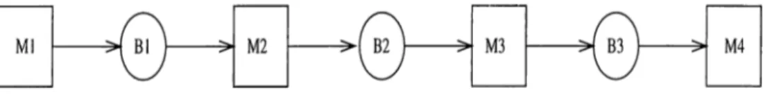
A tra.nsfer line is a rnanulacturing system which is usually used in ma.ss production systems. It is defined as a collection of linear machines (7V/|, /V/2,...,Mk) separated by buffer storages (Bi, B2 , ... , Bk-\). Parts flow from outside the system to Mi then to Bl then to M2, and so forth until it reaches Mk after which it leaves. Figure 2.1 depicts a four-machine trarisfer line separated by three buffers. The rectangles represent machines and the ovals represent Iruffers.

CHAPTER 2. REVIEW OF SERIAL PRODUCTION LINES

Figure 2.1: Four-Machine Transfer Line

Machines’ behaviours cire not perfectly predictcible. All machines require unpredictable, or predictable but not constant amount of time to complete their operations. Furthermore, all machines eventually fail and their repair times and the time between failures are not also perfectly predictable. This irregularity has the potential for disrupting the operations of not only adjacent machines but also machines further away. Therefore, iDuffer storages a,re used to reduce this potential.

When a failure occurs, or when a machine tcikes an exceptionally long time to complete an operation, the level in the adjacent upstream storcige may rise. If the disruption persist long enough that storage fills up cirid forces the upstream machine to stop processing parts. Such a forced-down machine is said to Ije blocked. Similarly, the level of adjacent downstream storage may fall during a failure, as the downstrecun mcichines drain its contents. If the failure persists long enough, the adjacent downstream storage is depleted and the downstrea.m nmchine stops processing parts. Such a forced down machine is called starved or idle.

Interstage buffer storciges partially decouple cidjacent machines. Since mcichine failures are inevitcible, buffer storages are used to reduce the effects of the failures of machines on the operations of other nicichines. When the buffer storciges are full or empty, the decoupling effect can not take place. When the downstrecun buffer is full, upstream machine can not send a part to tlie buffer and when the upstream buffer is empty, downstrem macliine can not take a part from the buffer when it needs to process. By supplying higli ccipacity buffer storages, probability of storages being empty or full are reduced. However, the disadvantage of high capacity buffer storages is the amount of average in-process inventory. As buffer sizes increase, more work-in process (WIP) inventory ciccumuhites between processing stages.

Work-in process, or WIP is undesirable. Gershwin[10] states the drawbacks of WIP inventory as ;

i) ¡t costs money to create, hut as long as it sits in buffers, it generates no

revenue.

ii) the average held time is proportional to the average amount ol inventory iii) inventory in a factory or a warehouse are vulnerable to damage or

shrinkage. The more items and the more time they spend, the more vulnerable they are.

iv) the space and the material handling equipment needed for inventory costs

money.

CHAPTER 2. REVIEW OE SERIAL PRODUCTION LINES 5

An in-process inventory can affect the production rate if the line is close to balanced. If the line is not balanced, even infinite buffers will have very suiall (dfects on the production rate. The size of the buffers should also be calculated cis the number of parts one nearby machine could make while another nearljy machine is down[10].

The factors that limit the production rate of a serial line are unrelial)le machines and hick of synchronization. Unreliable machines cause the line to stop the production. All other machines wait the unreliable machines to be repaired. To synchronize the system, Irequency and duration of unsynchronized (ivents may be reduced or in-process buffers may be installed. The place and tlie size of an in-process buffer is a design problem cind it is very important to increase the sjestem performance and to decrease the number of in-process inventory.

Another feciture of the transfer lines is the Vciricibility. There are few papers dealing with Vciriability of production lines[10j. Almost all of them calculate' the steady-state performance measures. However, variability of the system is very importcint. A stable system with low production rate may be preter-red to an unstable system with high production rcite. In other words, the less variability in the system, the more desirable the system is.

CHAPTER 2. REVIEW OE SERIAL PRODUCTION LINES

A common technique while modeling the transfer lines is M arkov-Chain representation. In this technique, all states of the system and their trcuisition probcibilities are defined. While obtaining the steady-sta.te probabilities, different methods are used. Another technique is decom position metliod. In this method, line is decomposed into two-stages which are the small ixipresentations of the exact model. When all these methods are ineffective in modeling the transfer lines, sim ulation is used. Simulation is a powerful technique used in modeling and also in experiments done for different parameters of the system.

2.1.1

D ifficu lties o f th e M arkov-C hain A p p roach

Markov-Chain models of the transfer lines iire difficult to treat because of their large state spaces and their in-decomposability.

The Mcirkov-Chain representation of a A;-niachine line with k — 1 buffers has M distinct states [10], where

k~i

M = 2^ n ^ ¿=0

an d Ni is the size of buffer storage Bi.

'I'hese models are not decomposable that is, portions of the system can not be treated as though they cire isolated from other portions. Approximate decompositions are derived, but no exact decomposition exists.

2.2

In ven tory P u ll S y stem

The traditional method of moving matericd is to push the required material down onto the shop floor, according to the production phui. A .lust in 'I'inie ap|)roach converts traditional shop floor control from a push system to a pull system for controlling inventories of materials and subassemblies.

In the push system, the finished-products (and customer orders) create computer planned orders within MRP, calculated to meet the requirement of the forecasts, orders, and associated subassemblies and components. These orders are converted into firm, planned orders that authorize the purchase of components and determine planning capacity requirement. When tlie order is locided to the shop floor it becomes a work order. At this point, components are allocated from inventory to meet the needs of this new work order. When components move onto the shoj) floor, a pick list is printed, parts are picked from component stores, and all peU’ts are moved to the shop floor ready to be manufactured. This traditional approach is called a ’’push” system, because materials cire pushed onto the shop floor based on the production plan c\,s it is seen from Figure 2.2.

CHAPTER 2. REVIEW OE SERIAL PRODUCTION LINES 7

Part Movement

Figure 2.2: Push Production System

A .lust in Time approach uses a ’’pull” system. A customer order appears at the end of the production line, and required materials are issued to the sliop floor a.s the operator request. The requesting of materials CcUi be done in a number of different ways, including the famous Kanbcui Method.

2.2.1

T h e P u ll S y stem

A pure pull system is initiated by a customer order. The supervisor on the final assembly line or at the final manufacturing station will ’’pull” the subassemblies required to complete the order from upstream workcells. The upstream workcells will pull subassemblies and components trom lower level cells, the Wcirehouse or suppliers (see Figure 2.3). For pull systems to work

CHAPTER 2. REVIEW OE SERIAL PRODUCTION LINES

cleaI l l y and precisely, very short manufacturing times and uniform demands to

the factory are required. In practice, this approcvch needs to be modified when there is a wide variety of products or when production cycle times must be

One widely used practice is to maintain small inventories of subassemblies and components on the shop floor in front of a work center. Subassemblies are stored in standard containers that always contain a specific quantity. When a downstream work center requires ci subasseiribly, the container is moved from the producing cell to the user cell. The user cell will I'eturn the empty contciiner to the producing cell, which then makes more of the subassembly to fill the returned container. Theoretically a container quantity will be equivalent to the amount used by the downstream work center; in reality, a little safety stock is also provided.

Inlormiition

Part Movement

Figure 2.3: Pull Production System

2.2.2

K anbans and Signals

A number of methods Ccin sigmd the movement of parts and subasseml)li('s to a downstreiun work center. The most well known method is the use ol Kanbcin cards. This method, developed originally by Toyota as a part of its (|uest for efficient manufacturing, requires the use of cards that are passed from one work cell to another. The word Kanban is Japcinese for card or ticket.

'I'here are two varieties of the Kanban method: one card or two card. 'I'lie two-card method has a production card cind a move card. The move card authorizes the transfer of one container of components from the supplying work center to the using work center. The production card authorizes the supplying work center to make another container of components.

The one-card system can be used in less complex manufacturing environ­ ments such as when there is one type of product to manulacture in a serial |)roduction line. In this case the Kanban card acts as both a move card and a production card. The Kanban travels with a container from the supplying work center to the using work center.

When more components ¿ire required, the Kanban is sent bcick to the supplying work center; at that point, the Kanban authorizes both the moving of iriiiterial cind the production of a new container quantity.

An interesting and useful phenomenon of a Kanban system is that WIP inventory level can be directly controlled through Kcinbans. Work-in-process inventory is directly related to the number of Kanbans on the floor.

Some more sophisticated cornpiinies make use of electronic Kanbans. This technique does not require any cards as such because any inlbrination recpiired to pull material from the prior cell or the warehouse is provided electronically. 'I'lie operator has a small computer terminal in the cell, enters the part number of the component or subassembly required, and triggers the supplying location to move the material.

2.2.3

A d van tages o f P u ll S y stem s

Advantages of Pull systems can be summarized from Maskell [18] as:

CHAPTER 2. REVIEW OF SERIAL PRODUCTION LINES 9

i)

CHAPTER 2. REVIEW OF SERIAL PRODUCTION LINES 10

production process. On the other hand, the medium and longer term planning underlying the simplicity of many Just in Time techni(|ues includes a great deal of planning cincl attention to detail. The availability of sufficient production resources, the purchase order of ra.vv material and components, production quality, shop floor layout and container quantities must all be right for a pull system to be effective.

ii) Another result of using demand pull as the primary production control method is tlmt more products iire produced. There is an intangible but very strong relationship between excess WIP and poor productivity. When the shop floor is full of large batches of semi completed asscmiljlies, operators may be confused as to what they should be working on and when.

iii) The big cidvcintage of a pull system is that only the material required

to mevke products is moved onto the shop floor. There is no excess or unneeded inventory; no waste. Pulling material answers the fundamental questions of when to manufacture a subassembly or buy a component a.nd how much to make. Pulling does not rely on forecasts, run times or lra.tch quantities.

iv) Despite the fact that some work centers ci.re operating at less than full rate, the amount of product produced is higher than wheji each workcenter is loaded 100% through a push system. This rate is sometimes spoken as a. "drum beat” of manufacturing l)ecause material flows through the factory at a. constant velocity; there is a predictable rhythm to the process resulting in a larger volume of finished products.

2 .2 .4

D isad van tages o f P u ll S y stem s

In addition to requiring short lead times cuid predictable (stable) demand, a pull system requires that there are no conflicting priorities within the production schedule. Just-in-Time manufacturers employ a numl:)er of

CHAPTER 2. REVIEW OE SERIAL PRODUCTION LINES 11

toichniques to alleviate priority conflicts. A key to the resolution of conflicts is flexibility of people and flexibility of machinery.

In the short term, the problem of priorities has to be overcome by keeping a.dditional inventory of assemblies produced by the affected work center.

Shortly :

i) A Pull system requires short lecid times and small production lots, which require fast setups.

ii) A Pull system requires flexibility of people and equipment so that changing requirements can be accommodated.

iii) A Pull system can theoretically be used with any kind of shop floor layout, Init is most effective in conjunction with a cellular type of layout.

iv) A Pull system reciuires total quality assuarance because a. quality failure at one cell can stop the entire production process.

v) A Pull system requires preventive rnaintencince rather than the mainte­ nance after machine break down.

2.3

L iteratu re R ev iew

2.3.1 A u to m a tic Transfer L ines

Automatic transfer lines phiy an important role in mass production systems. An automatic transfer line is defined as a number of automated nmchkies intcigrated into one system by a common automated transfer mechanism. Workpieces (parts) enter the system through the first machine and after being [processed by all the machines in a sequential order they leave the system through the last machine. Transfer of parts from one machine to the next

CHAPTER 2. REVIEW OF SERIAL PRODUCTION LINES 12

are synchronized to take place at the scirne time. In a synchronized transfer line, the hiilure of a single machine can cause the stoppage of the whole system resulting in the loss of production. This problem, however, can partially be solved if buffer storages are provided between the machines.

In the literciture, there cire lots of works of transfer lines. They are different in the cissumptions of models, such cis relicible or unreliable machines; machines with hnite buffers or mcichines with inhnite buffers; distributions of the downtimes, cycle times, repair times etc. However, they have a common feature of thcit cill systems are modeled under the Push policy. There are few papers dealing with automatic transfer lines under Pull policy.

The two-stage transfer lines are solved by Markov-Chciin easily. When the number of stages is increased, the number of states increases greatly and the solution with Markov Chain becomes very difficult. Some approximation techniques to solve N-stage transfer lines are developed cuid reported in the literciture.

Shantikumar cind Tien[26] have analyzed two-stage synchronized automatic transfer line where workpiece transfer at all stages is synchronized to occur at the same time. The model is represented as Markov-Chain. However, tlie method used to solve this Mcirkov-Chain is different from solving the set of equations

x P = X (i^ 1)

xe = 1 (2.2)

where x is stecidy-state probability vector of Markov-Chain. The algoritlim to solve the Markov-Chain representation of the model is given in the paper. It is also suggested that the idea of providing buffer storage is to minimize the second stage idleness and to reduce the probability of first stcige being blocked.

Anal3^sis of some extensions of this model using cin efficient interpolation

approximation is discussed in Ignall and Silver[14] and using simulation is described by Ho et al.[12, 13]. Okarnura and Yarnashina[22] luive considered the same two stage transfer line except they assumed that units are scrapped

CHAFTER 2. REVIEW OF SERIAL PRODUCTION LINES 13

whenever a machine processing it fails.

.Jafari and Shantikurnar[15] hcive modeled N-stcige transfer lines as Markov- (Jhain.

Figure 2.4: N-Stage Transfer Line

N-stage ... Mu-uHn-i, t r a n s f e r lines (see Figure 2.4)

are modeled as Markov-Chain by observing its state just after ecich transfer of parts. Because of the large state space, an approximate model called Decomposition-Aggregation Method is used. In this method,

Lrrsl two-stcige system is represented as {M\^ M2)

Second two-stage system is represented as (RMi, B2, Ms) where RiMi is the equivalent stage which replaces {Mi, By, M2)

Third two-stage system is represented as {IIM2, B3, M.y) where R M2 is the equivalent sttige which rephices {My, By, M2, B2, Ms) or {RMy, B2, Ms).

In general, j t h two stage system (for j - I...N - 1) is represented as {RMj - \ , Bj,Mj+y) where RMj-y is defined as equivalent stage which replaces {My, By , ...Mj-y, B „ M j ) for j = 2...N - 1.

'I’his problem is solved through a series of iterative steps. The algorithm is given in the paper of .Fifari and Shantikunicir[I5].

A similar model with no scrapping has been analysized by Sevastyanov [24], Buza.cott[3, 4] , Sheskin[27], Gershwin[ll]. The model of a rnultistcrge transler line with scrapping has been considered by Shanthikumar[25j.

CHAPTER. 2. REVIEW OF SERIAL PRODUCTION LINES

uptime and downtime distributions. It is assumed that the distribution of uptime and downtimes of each stage are of phase type. Using the pluvse structure of the underlying distributions, the system is modeled as a Markov- ( 'liain.

(Jonway et al.[6] investigates the behaviour of asyncronous lines ¿uid e.x:plores the distribution and quantity of work in process (WIP) inventory tha,t accumulates. Simple, generic production systems are studied to gain insight into the l:)ehaviour of more complex systems. The paper is concluded witli the suggestion that buffers between workstations increase system capacity, but with sharply diminishing returns. Positions as well as capacity of buffers are important.

2.3.2

P u ll S y stem s

Muckstadt and Tciyur[20, 21] have shown the difference between Traditional Kanban Control System (TKCS) and Constant-Work-in-Process (CJONWIP) type control system. If the serial production line consists of M rnacliines arranged in a series of (or in tcindem), these M machines are partitioned into N cells. If all the M machines are in the same cell, we have a (JONWIP type control system; if on the other hand, there are a total of M cells, each cell containing exactly one machine, then we have a Traditional Kanban Control System (TKCS). In other words, if N{Mi , ....M2){Ci, ....,Cn)(B) denotes a serial production line with N cells. Mi machines in cell i, Ci white kanbans in cell i, i = I...N, and B colored Ccuxls that circulate throughout the shop floor, CONWIP is a l /{M) / {C) / {. ) system, and TKCS is a yW/(l,..., l) /( ( 7 i,...., (7m)/(.) system. The difference between the model that we will construct and these two types of inventory control systems defined above is that the mechanism of the two control systems mentioned above is pull between cells cuid push within a cell. However, in our model that we will construct, mechanism is pull for only the last cell and the other cells operates according to the requests made in this last cell.

CHAPTER 2. REVIEW OE SERIAL PRODUCTION LINES 15

Spearman and Zazanis[28] examined the behaviour of push and pull production systems in an attem pt to explain the apparent superior performance of pull systems. Three conjectures are considered in the paper; that pull systems Inwe less congestion; thcvt pull systems are inherently easier to control; and that the benefits of a pull environment owe more to the fact tliat WIP is bounded than to the practice of pulling everywhere. Moreover, a control strategy that has i:)ush and pull characteristics is identified a.nd it is shown that this hybrid system outperforms both pure push and [)ure [)ull systems. Corbett[7] focuses exclusively on model based approciches in studying pull systems. Eventhough aucilytical models such as linear programming formulations or queing approximations exist, it is concluded that the inherent complexity of pull systems makes simulation an essential tool in studying them. Slobodow[29] studied the implementation of inventory pull (kanban) systems with simulation modeling as a means to quantitatively design such a system. Tlie simulation results confirmed the fecisibility of the pull system. The pull system caused an acceptably low amount of stcirvation in the machining lines and with this system, phmt-wide inventory was reduced by 48%. Galbraith et al.[9] solves the problem of providing decision support lor the transition from a traditional push production system to a pull system design.

MerciJ and Erkip[19] proposed a design methodology which addresses the design decisions involved in the design of an idecd .JIT production line operating in an uncertain environment. Durmusoglu[8] describes the performance of tlie pull and push-systems in a celluar rncuiufacturing environment through an industrial appliccition Cci.se. Rarnudhin and Rochette[23] evaluated tlic perlbrmance of a .JIT production system in the assembly department of an electronic equipment manufacturer where production is highly unstable. Then a pull type production system tailored to the specific needs of the problem at hcuid was developed. Lingayat and Mittenthal[17] suggested that the performance of a pull system deteriorates rapidly under non-ideal conditions, suggesting that a .JIT system shouldn’t be blindly implemented. An incremental approach based on order release wa.s suggested as a, step towards irnplementing .JIT manufacturing.

CHAPTER. 2. REVIEW OE SERIAL PRODUCTION LINES

Askiii, Mitwasi and Goldberg[2] developed a stochastic model to determine the number of kanbans in multi item JIT systems. They also used simulation to check the accuracy of the model. Wcuig and Wang[30] developed a procedure to decompose a complex JIT system into a number of station pairs and they developed an algorithm to determine the optimal number of kanban for ea.cli pair of stations. Andijcuii and Clark[l] proposed different rules for allocating kanbans to maximize system performance for a pull system considering both i.hroughput rate and WIP levels. Co and Jacopson[5] developixl a recursive! function which computes the number of kanbans required for all stages of serial |)roduction system. This function is used to compute a. lower bound on the expected fill rale for an cu-bitrciry kanban assignment.

As it is seen from the above survey that transfer lines and pull systems a,i-e tlie concepts that were usually worked on separately. There are few works about the transfer lines and pull systems together. However, these works are also l)ased on different assumptions from the ones used in our model. In addition, constructing the Markov Chain model of this combined model is also a very good contribution to the literature.. In the following chapters of this study, we will see the details of our analytical and simulation model.

C h a p ter 3

M o d elin g o f th e P u ll S y ste m s

'[’lie JVIarkov-Chain model of the two-stage transfer line with capacitated liulfers under pull environment are constructed in this chapter. Although, most of the assumptions of the model with buffer sizes of 1 and those of the model with Iniffer sizes of more than two are the same, there are some small differences vvhicli rna.y change the performance of the system.

3.1

D escrip tio n o f M od el 1

MACHINE 1 BUFFER 1 MACHINE 2 BUFFER 2

Figure 3.1: Pull Production System

CHAPTER 3. MODELING OF THE PULL SYSTEMS 1 8

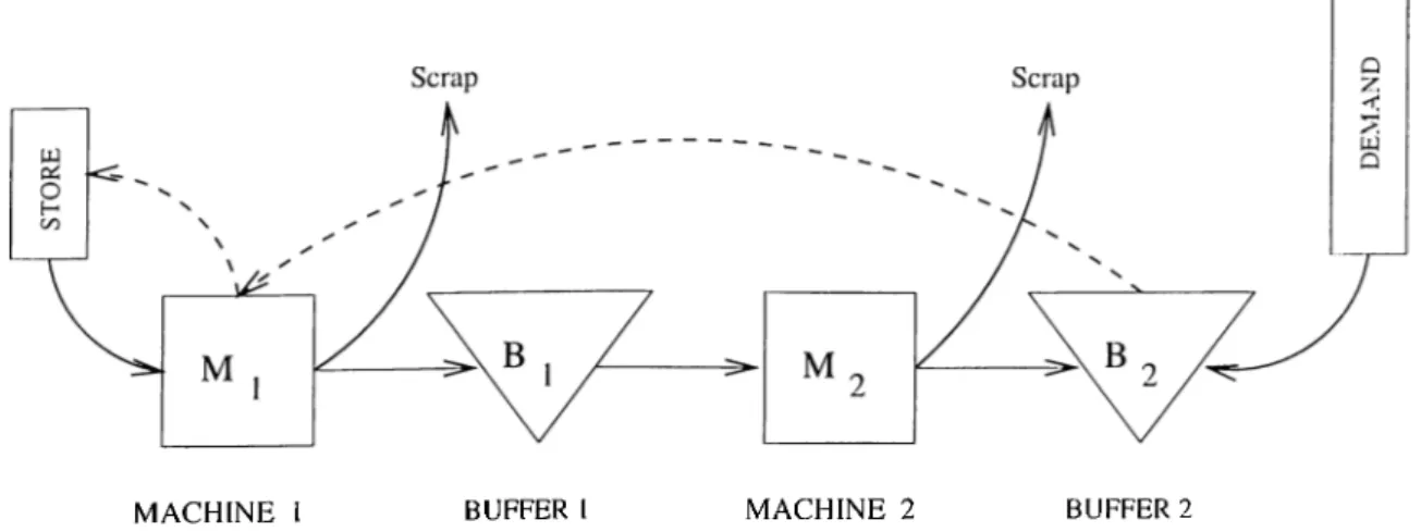
A simple two-stage pull production system is depicted in Figure 3.1 and the assumptions of the model constructed are given below.

A ssum ptions :

• System is an automatic transfer line with fixed cycle time. • System is observed cifter the transfer of e£).ch unit

• Demand arrives at the beginning of each cycle according to Poisson distribution with pcirarneter A.

• When the demand arrives, if there is an item in the last buffer, it takes that item, if there is no item in the bist buffer, demand is not satisfied (no bcicklogging).

• Afl mcichine processing times cire constant. • 'f'here is no shortcige of material on the store. • Buffer capacities are one (i.e., Ni = 1 and N2 = 1).

• /'A machine breciks down only when it is processing an item.

• Machine i breaks down according to geometric distribution with parameter Pi (i = 1,2)

P{X, = . r } - ( l - p i ) ’- V (3.1)

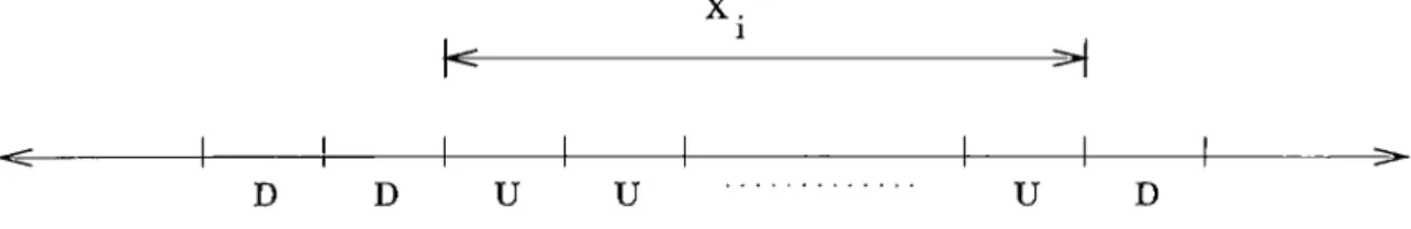
where Xi is the number of cycle times for machine i from the time that ma.chine is repaired to the time that nicichine breaks down as it is seen from Figure 3.2. Here, U represents the uptime period and D represents the downtime period of the machine.

CHAPTER 3. MODELING OE THE PULL SYSTEMS 1 9

X.

D D U U U D

Figure 3.2: Time horizon for the states of an up system

• Machine i is repaired according to geometric distribution with parameter <H ('i = 1,2)

P{Y^} = { l - c u r - ' q i (3.2) where Yi is the number of cycle times in which machine is down (see Figure 3.3.)

Y.

--- b

U U D D --- D U

Figure 3.3: Time horizon for the sta.tes of a down system

• When the machine i is repciired, the item on that machine is scrapired with probability ri ( i = 1,2).

Param eters :

c : cycle time

pi : probability tluit machine i breaks down during the cycle given that it was operative cit the end of the previous cycle.

Vi : probability tluit pcirt j will be scriipped when the machine i breaks down and then repaired.

1 _ : probability that pcirt j will be completed on machine i aitei’ the

CHAPrEB, 3. MODELING OF THE PULL SYSTEMS 2 0

1/(·/,: : mean of the repair time

(¡i : probability that repair is completed in a cycle given thcit machine i (i = 1,2) broke down or was under repair during the previous cycle (at the end of the previous cycle)

d : probability of one or more demand arrives

(i = 1 — (3.2)

This system works in the pull environment. When one or more demand arrives, one of the demands is satisfied if there is a part in the last buffer and tlie remaining demands are lost. When a ])art is removed through the demand the last buffer becomes empty and production of a new part is instructed for machine 1. Machine 1 gets this instruction and asks a pcirt from the store. When a new part comes to the machine 1, processing on that part starts. During thcit process, machine may break down. If it breaks down, a repair stage starts. Machine stays at the repair stage ciccording to a geometric distribution. After the machine is repaired, the part on that machine might be scrapped or it is sent to downstream buffer. In the latter case, if the downstream buffer is full, machine becomes Irlocked. If a downstream machine can not, find a, pa.rt to process on the upstream buffer, it waits as idle.

3.1.1

N o ta tio n

States:

U ; represents the state of being operative (up) for a machine

D : represents the state of being down or under repair for a machine B : represents the state of being blocked for a machine

CHAPTER 3. MODELING OF THE PULL SYSTEMS 2 1

Any state of the system (or model) is represented in the four tuples of (,S'i, A^i, S2, N2) where

,S'i represents the state of machine 1 and takes the values of {U,D ,B} N\ represents the state of buffer 1 and takes the values of {0,1}

S'2 represents the state of machine 2 and takes the values of {/7, D, /7, / ) N2 represents the state of buffer 2 and takes the values of {0,1)

To represent the Markov-Chain model of the system, all states of the model must be obtained. If the states are written in blocks, it becomes very easy to obtain a transition probability miitrix in block-diagonal form. The block diagonal matrix saves time in computation and it is also easier to write a computer program to solve this Markov-Chain representation.

VVe describe the blocks of the states in three different blocks for the buffer size of one. They cire described as follows :

Xj : represents the set of states where the state of machine 2 is idle. .\''o : represents the set of states where the state of buffer 1 is zero A'l : represents the set of stcites where the state of buffer 1 is one

If all states are shown in their respective blocks.

X i= {(/7,0, / , 0), ( D, 0, / , 0), {U, 0, /, 1), (D, 0, / , 1)}

A'„= {[(7/, 0,77,0), (7/, 0, T>, 0), {D, 0, U, 0), {D, 0, D, 0)],

[(7/,0,77,1), (7/, 0,77,1), (/7,0,7/, 1 ),(D ,0 ,D ,1 ), (7/, 0 ,£ i,l), (77,0,77,1)]}

CHAPTER 3. A40DELING OF THE PULL SYSTEMS

[W, I, c/, 1), ((7. l , D, l ) A D , l , U , l ) AD, l, D, 1), (U, 1. B, 1). (A 1, B, I),

( B , l , / J , l ) , ( f l , l , ( 7 , l ) , ( B . l . A l ) l )

Block Dicigonal form of the probability transition matrix is shown in Figure 3.4. When writing the states in blocks, the order given above is preserved.

A few examples cire given below to represent the computation of getting the probability of going to a state from another state.

Exam ple 1 :

P ro b {(/7 ,0, D, 1) ( D ,0 ,/ ,0 ) } = P ro b jm ach in e 1 breaks down} * Prob{nici,chine 2 is repaired)*P ro!){the p art is scrapped after nicichine2 is repaired}*P rob(one or m ore dem and arrives)

= Pi * <l2 * >'2 * d

E xam ple 2:

Prob{(f/, 1, 1) =>■ 1,7?, 1)} = Prob{mi\.chine 1 does not brecik down}*Prob{ma.chi 2 does not breiik down)*Prob{no demand cirrives)

me

CHAPTER 3. MODELING OF THE PULL SYSTEMS 23

l''igui'e 3.4: ]31ock diagonal form of the Markov Chain Model for /V = 1

E xam ple 3:

Prob{(/9,1, D, 1) ^ (U, 1, U, 1)} = Probjmachine f is repaired}*Prob{tlie part on nicichine 1 is not scrapped}*Prob{rnachine 2 is repaired}*Prob{(the part on ma.chine 2 is scrapped and no demand arrives) or (the part on macliine 2 is not scrapped and one or more demand arrives}

CHAPTER 3. MODELING OF THE PULL SYSTEMS 24

'I'wo block probability matrices are shown below to get a better idea about the model description as a Markov-Chain.

E xam ple 4:

Probability trcuisition matrix of going from the stcites of X j to the states of X, is shown below.

A n =

0 _Pi 0 0

f/P’i 0 0

0 dpi 0 (1 - d)pi

qii'id {;i - qi)d - d

E xam ple 5 :

As another example, the probability transition nmtrix of going from the statcis of A'o to the states of X i is shown below.

CHAPTER 3. MODELING OE THE PULL SYSTEMS r\(U 0 0 0 0 0 0 0 Pi </2^2 0 0 0 0 <hr\q2r2 (1 - q\)q2r2 <Zi'’i<'/2(l - 7-2) 0 Piq2r2d 0 0 0 qiriO - 1)2)d P ii p 2 ) Pi 172(1 - 1-2) (1 - f/i)(l - P2) (1 - <7 1)1/2 ( 1 - /-i) P i(l - p2)d 7>i<72[(1 - r 2 )d + r 2 (l - d)] (1 - ^/i)(l - P2)d

<'/i''-iC/2?’2(/ (1 - q\)q2r2d <'/i?-i</2'’2(l - d) (1 - <7i)</2[r2(l - d.) + (1 - ■/•2)c/]

0 0 0 0 0 qiVid P\d (1 - <7i)<:'^

3.1.2

M o d el S olu tion

his Mai'kov-Chain model is solved by using the set of equations

x P = X xe — 1

(3.4) (3.5)

where x is the steady-state probabilities of each state of the model and c is the unit vector. Since the number of states is small for the buffer size of one, there is no difficulty in solving this equation set.

We have written a program in the package Maple to solve this set of eiiuations. Using computer program makes the life ea,sy since you can change

CHAPTER 3. hdODELING OE THE PULL SYSTEMS 26

parameters at the initial step, compute the steady-state probabilities of the states and then you can compute the performances of the system by using these probahilities.

'['lie algorithm of the program is provided below. Since the buffer size is one and state space is small, transition probabilities are entered directly, there is no need to generate it automatically.

A lgorithm :

Step 1 : Generate A n , Aw, A n block matrices by directly writing the transition

probabilities.

Step 2 : Generate Aoi, Ago, Aqi block matrices by directly writing the transition probabilities.

Step 3 : Generate A n , Am, A n block matrices by directly writing the transition

probabilities.

Step 4 : Gornbine all block-matrices sequentially (i.e.. A n , Am,An, Am,

/loo,2loi, 2li/,/lio,2ln) to obtain a block-diagonal matrix /^.

Step 5 : Solve the set of equations 3.4 and 3.5 by using

x{P - /) = 0

xe — 1

E xp erim ents :

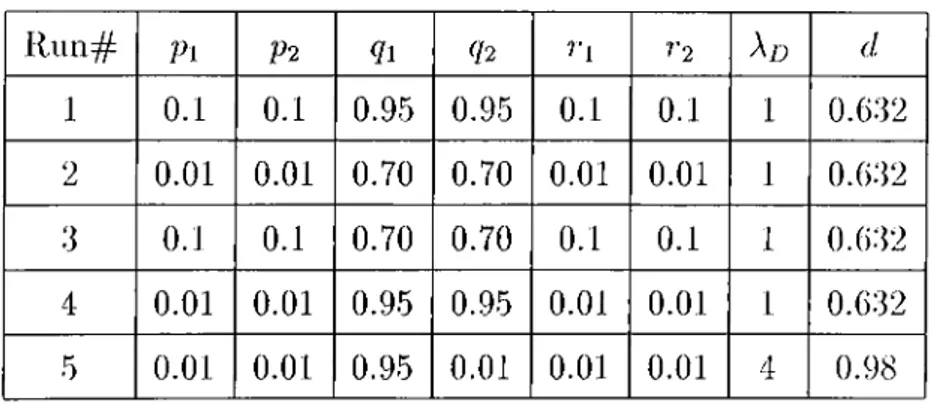
By using different parameters, we have designed an experiment to see the relations Ijetween parameters of the model and to compute the pertbrmance measures. The table of parameters used in the experiment is shown below :

CHAPTER 3. MODELING OF THE PULL SYSTEMS 27 R un# Pi P2 _<Z1 <I2 ^1 V2 Ad d 1 0.1 0.1 0.95 0.95 0.1 0.1 1 0.632 2 0.01 0.01 0.70 0.70 0.01 0.01 1 0.632 3 0.1 0.1 0.70 0.70 0.1 0.1 1 0.632 4 0.01 0.01 0.95 0.95 0.01 0.01 1 0.632 5 0.01 0.01 0.95 0.01 0.01 0.01 4 0.98

Table 3.1: Parameters used in Experiment 1

J3y using these parameters, we have computed dilFerent performance mecisures. The performance measures used and their formulas are given below:

a) a = Percentage of Demand satisfied = Prob { last buffer size is one } 1)) 1) = Expected numbers in the buffers = 1 * Prob {no. of pa.rts on the

buffers is one} + 2* Prob (no of parts on the buffer is two j

c) C] = Prob (Machine 1 is blocked ) = Total probability of the states that machine 1 is in B stcite

(■■2 =Prob (Mcichine 2 is blocked ) = Total probability of the states that machine 2 is in B state.

d) (1 = Prol){machine 2 is idle} =Total probability of states that machine 2 is in / state.

e) C] = Percentage of scrapping on mcxchine 1 = n * Prob {machine 1 is down }

e.2 = Percentage of scrapping on iruichine 2 = ?’2 * Prob {machine 2

is down}

f) /i - Percentage of uptime for machine 1 = Total probability of the states that machine 1 is in U state.

CHAPTER 3. MODELING OF THE PULL SYSTEMS 2 8

/ 2 = Percentage of uptime for machine 2 = Total probability of the

states that rricichine 2 is in 17 state.

'lie results are shown in the table below :

Run# a b Cl C2 d ei ('2 h h 1 0.9464 1.8467 0.3241 0.3234 7.4 *10-3 6.45 * 10-3 6.38* 10-3 0.6117) 0.60.6.') 2 0.99 1.977 0.3636 0.3623 0.0014 8.9* 10-·^ 8.8* 10-3 0.62 0.6272 3 0.9201 1.7867 0.3221 0.3088 0.0203 8.5* 10-3 8.4 * 10-3 0..6933 0..6873 4 0.9916 1.8771 0.3066 0.3604 6.3* 10-3 6.6* 10-·^ 6.-5* 10-3 0.6273 0.6267 5 0.9173 1.1123 .5.2 * 10-3 0.0168 0.0747 9.48 * 10- ‘ 9.4*10-·^ 0.899 0.899

Table 3.2: Results for Experiment 1

in an another experiment, the parameters and the results for the perlbrmance measures explained before are shown in Table 3.3. a.nd 'I'alile 3.4. respectively. R u n# _{P I} P2 <11 <72 r i »'2 ^E> 1 0.01 0.1 0.7 0.95 0.01 0.1 1 2 0.01 0.1 0.7 0.95 0.01 0.1 4 .. 3 0.01 0.1 0.7 0.95 0.01 0.1 8 4 0.1 0.01 0.95 0.70 0.1 0.01 1 5 0.1 0.01 0.95 0.70 0.1 0.01 4 6 0.1 0.01 0.95 0.70 0.1 0.01 4 7 0.001 0.15 0.70 0.90 0.90 0.05 1 8 0.001 0.15 0.70 0.90 0.90 0.05 4 9 0.001 0.15 0.70 0.90 0.90 0.05 8 10 0.15 0.001 0.90 0.70 0.05 0.90 1 11 0.15 0.001 0.90 0.70 0.05 0.90 4 12 0.15 0.001 0.90 0.70 0.05 0.90 8

CHAPTER 3. MODELING OE THE PULL SYSTEMS 29 Ru n # ^2 1 7.7 ♦ 10“ -^ 1.26 ♦ 10" 00776 6.48 ♦ 10“ "^ 1.04 ♦ 10-3 0.3557 0.1470 7.12 ♦ 10" Table .3.4: Re,suits tbr Experiment 2

In the following figures, each bar represents the value of the chosen performance measnre for a specific run. For example, the number [1,4] above the bars show that the first bar under this number shows the value for R u n # l a.ncl the second bar under this number shows the value for Run#4.

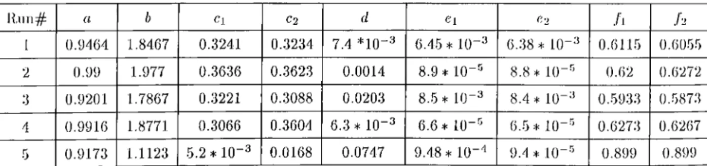
in Figure 3..9, we see that when we put more reliable mcichine with p2=0.01 and r2=0.01 but with q2=0.7 (i.e., waits in repair state more) at the end of the line in case 1 (ie.. Run # 1-4) and with p=0.001 and ?’=0.9 and (/—QJ in case 2 (ie., Run # 7-10) , the percentage of demand satisfied increases. This is because of the fact thcxt when demand arrives, the last machine is found more operative and sending finished parts to the buffer in that case. However, there is an interesting result that, when the demand increases greatly with respect to tlie l)uffer sizes, in our case d=8 cuid A^=l, there is no difference in |)ercentage of demand satisfied.

When we again put the more reliable machine at the end of the tine, the expected total number of parts in the buffers decreases as it is seen in Figure 3.6. If we increase derrumd greatly, such as d=8, the difference between these two cases becomes more apperant. This is because of the fact that when the more reliable nicichine is in the upstream cind the other mcichine is in the downstream , upstream machine becomes blocked quickly cind the parts on l)uffer 1 piles up. This increases the average number in the buffers.

As we have said before, when the more reliable machine is put at the downstrecim and the other mcichine at the upstream, percentage ol upstream

CHAPTER 3. MODELING OE THE PULL SYSTEMS 30

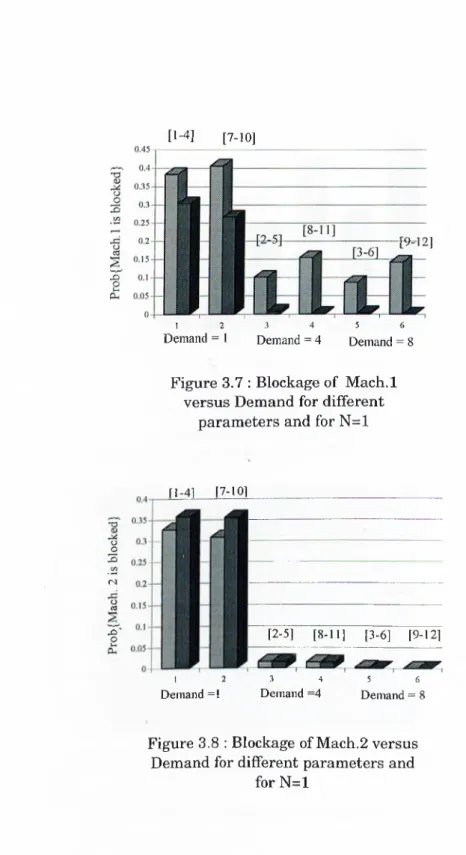
nia,chine’s blockage decreases (see Figure 3.7) and percentcige of downstream nmchine’s blockage increases (see Figure 3.8) since it is more reliable and rapid.

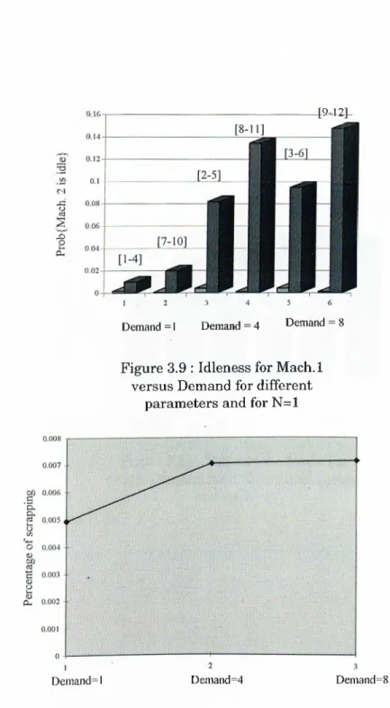
When the more reliable machine is in the downstream, the percentage of idleness increases sharply, since the unreliable machine can not send enough parts to the downstream buffer and makes the downstream machine idle (Figure 3.9).

'riie scrapping on Machine 1 and Machine 2 increases when demand increases (see Figure 3.10), but the slope of the figure decreases and levels at a fi.xed value. This may be because of the fact thcit, the machines reach up tlie fidl capacities and at the full capacity there is a fixed scrap percentage. So, at very large demands, the scrap percentage hits its limit.

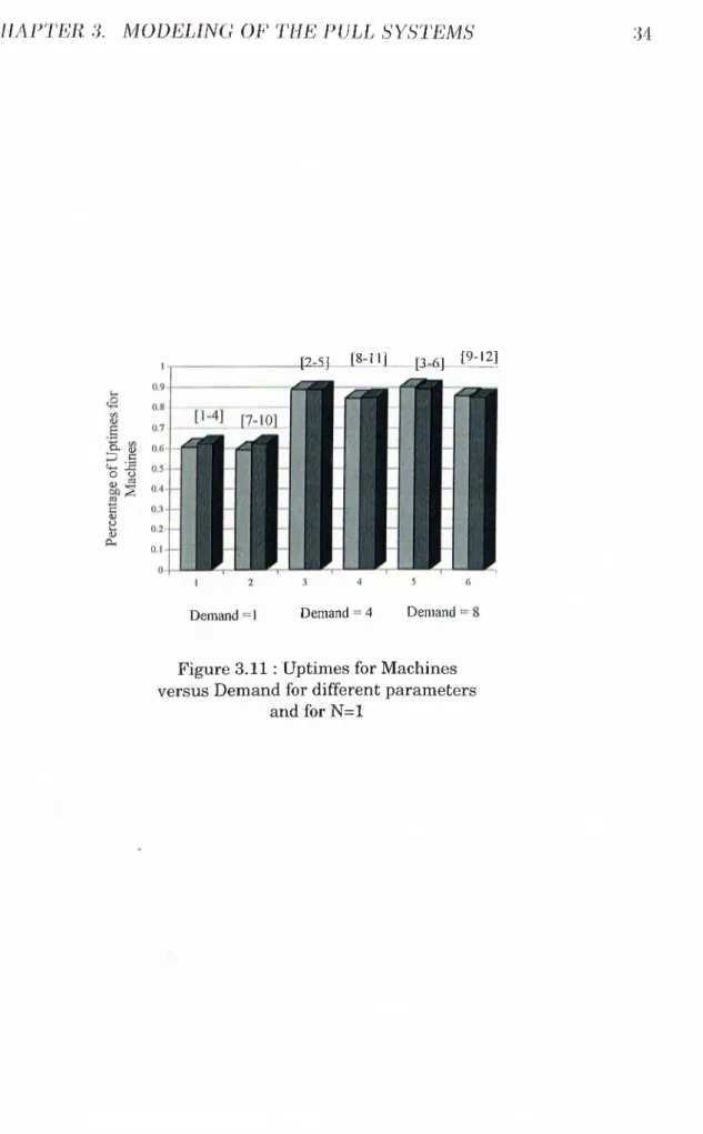
When we exchcuige the machines, the percenta.ge of uptime does not, clia very much for the Scirne machine (see Figure 3.11).The percentcige of uptime does not differ grecitly, when demands reach high values, such as d=4 or d=8.

CHAPTER 3. MODELING OE THE PULL SYSTEMS 3 1 <U pH ['-4 ] [7-10] 'TU_CL) C+H cj C/D nd g 0.95 3 4 5 (5 Demand = 4 Demand =8

Figure 3.5: Percentage of demand satisfied versus Demand for different parameters and for N=1

[1-41 [7-10] [2-5] [8-11] [9-12] t:_cd pH V-. ,(D CD fe I pa ^ CD T3 tl!_{o .s} o CD o -X 1.8 1.6 1.4 1.2 1 0.8 -0.6 0.4-0.2 0 -Demand = 1 3 4 5 Demand = 4 Demand =

Figure 3.6 : Expected number of parts versus Demand for different

CHAPTER 3. MODELING OE THE PULL SYSTEMS 32 [1-4] [7-10] [9-1-2] 1 2 Demand = 1 Demand = 4 5 6 Demand = 8

Figure 3.7 : Blockage of Mach.l versus Demand for different

parameters and for N=1

ri-41 [7-101 o o r4 o d Xi'_o 1 2 Demand =1 [2-5] [8-11] [3-6] [9-12] 5 6 Demand = 8 3 4 Demand =4

Figure 3.8 : Blockage of Mach.2 versus Demand for different parameters and

CHAPTER 3. MODELING OE THE PULL SYSTEMS 33

[9^11]-1 X)_o

Demand =1 Demand = 4 Demand 8

Figure 3.9 : Idleness for Mach.l versus Demand for different

parameters and for N=1

Demandai Demanded Demand=8

CHAPTER 3. MODELING OE THE PULL SYSTEMS 34 [2-5] [8-11]____p - 6 ] [9-12] ^ o .s o o (D ca C H) o

Demand =1 Demand = 4 Demand =

Figure 3.11 .‘ Uptimes for Machines versus Demand for different parameters

CHAPTER 3. MODELING OF THE PULL SYSTEMS 35

3.2

T w o S tage M od el w ith Buffer C ap acities

o f N iN > 2

)

MACHINE BUFFER MACHINE 2 BUFFER 2

N, > 2 N^> 2

Figure 3.12: Two Stage Model with buffer capacities of N > 2

Most of the assumptions of this two-stage model are same with the tliose of our previous two-stage model. However, there cire some differences in the assumptions which are given below :

• Buffer sizes are general (N > 2)

• Machine 1 can l)e in idle state because when the last buffer is full and nuichine 2 is ujr at the end of a cycle time, machine 2 l:)econies blocked and a new part can not be released from the store to the machine 1. Therefore, machine 1 waits idle until a command is sent from machine 2 when the blockage is removed.

• Number of states differ grecitly. If N represents the buffer size,

N i35i states where the state of rncichine 1 is idle) has N -|-1 states Xj.^ (set of states where the state of machine 2 is idle) has 2'''(At -)- 1) sta.t(-js

CHAFTER, 3. MODELING OE THE PULL SYSTEMS 36

Aq lifts 4:^{N “I” stcitcs

N ¡.0 Y i A N — 1) has 4*(N + l) + 2 states .Y/v has 6*(A^ + l ) + 3 states

• d-k Y k < N) represents the probability of k demand arrives

(4 = Prob{k demand arrives} = (A/A;!) * (0 < k < N — 1) N - l

diM ~ 1 — dk

k=0

To represent the states, we give an example of the state blocks for the buffer sizes of two.

Ab,= { (7 ,0 ,./? ,2 ),(/,l,i? ,2 ),(/,2 ,i? ,2 )}

AT,= { ( f / ,0 ,/,0 ) ,( A 0 ,/,0 ) ,( t/,0 ,/,l) ,( i:) ,( ) ,/,f ) ,( /7 ,0 ,/,2 ) ,( A 0 ,/,2 ) } A'o= {[(7,0, ¿7,0), (U, 0, D, 0), (D, 0,f/, 0), (D, 0, D, 0)], [((/, 0, 7,1), (U, 0, D, 1), (D, 0, U, 1), {D, 0, D, 1)], [(//, 0, f/, 2), (f/, 0, D, 2), (D, 0 ,7 ,2 ), (D, 0, /7,2), (/7,0, B, 2), (D, 0, B, 2)]} AT= {[(//, 1, U, 0), (U, 1 ,7 ,0 ), (D, 1,7,0), ( D, 1, D, 0)], [(/7,1, /7,1), (/7, l , D , 1), (D, 1, U, 1), (D, 1, D, 1)], [ ( /7 ,l,f 7 ,2 ) ,( / 7 ,l,D ,2 ) ,( A l,t / ,2 ) ,( A l ,A 2 ) ,( t /,l ,5 ,2 ) ,( 7 7 ,l,i i ,2 ) ) X , - {[(7,2, U, 0), (U, 2, D, 0), (D, 2 ,7 ,0 ), (D, 2, D, 0), (B, 2, /7,0), (/7,2, /7,0)], [(77,2,77,1), (7/, 2, D, 1), (D, 2,7/, 1), (D, 2,77, i), (B, 2,7/, 1), (77,2, /7, f )], [(7k 2,77,2), (7/, 2,77,2), (77,2,77,2), (77,2, /7,2), (7/, 2, B, 2), (77,2,77,2), (77,2,77,2), (77,2, U, 2), (7?, 2,77,2) }

The block diagonal form of the probability transition matrix is showii in l''igure 3.13. if we removed the first row and the first column of the blocks, we would obtain a pure block-diagonal matrix.

Cl [AFTER 3. MODELING OF THE PULL SYSTEMS 31 X .

X

0

X

N

X

X ,

A

A

0

0

0

A

I

I

X

A

A.

A.

0

0

A

A

A

0

0

A

X

N-l

0

0

0

0---A,

A

A

A

X

N

0

0

0

A

A,

^ I I

X

A

I

I

A

A

A

A

XiN

A

_{I| II}

l·'iguı■e 3.13: Block-Diagonal form of the Markov-Chain Model lor bulfei· sizes of N

CHAPTER 3. MODELING OF THE PULL SYSTEMS 38

To eci.se computations, we also break each block matrix into sub blocks. This eases writing a flexible computer program for any bufler sizes. Let us give some examples to show these block features.

E xam ple 6 : (I.0,B,2) (1.1,B,2) (1.2,B,2) (U,l,u,0) 0 0 0 (U,1,D,0) 0 0 0 (D,1,U,0) 0 0 0 (D,1,D,0) 0 0 0 (U,1,U,1) 0 0 0 (U,1,D,1) 0 0 0 (D,1,U,1) 0 0 0 (D,1,D,1) 0 0 0 (U,1,U,2) 0 0 (doPiP2)

(U,1,D,2) 0 0 (c/o?2(l - r2)(l - p-i))

(D,1,U,2) 0 -p->)do d.Q(n{l - n)(l - P2)

(d,i,d;2) 0 do<Ziri(?2(l - >’2) (doqiii - »-1)92(1 - »’2))

(U,1,B,2) 0 0 do(l -Pi)

(D,i,B,2) 0 doqivi do9i(l - »-i)

Table 3.5: Probability transition matrix from Xi model with N = 2

CHAPTER 3. MODELING OE THE PULL SYSTEMS 39

(U,0,1,0) (D,0,1,0) (U,0,1,1) (D,0,1,1) (U,0,l,2) (D,0,l,2)

(U,0,1,0) 0 Pi 0 0 0 0

(I),0,1,0) qiri _(T<Zi) 0 0 0 0

(U,0,I,1) 0 (di + d2)pi 0 P i(d) 0 0

(D,0,1,1) (di + d2) qi r i) (di + c/2)(l — qi) (d)qiri (c/)(l - qi) 0 0

(U,0,l,2) 0 P l d2 0 pidi 0 Pi(d)

(D,0,l,2) qirid2 (1 - ql)d2 qii'idi (1 - qi)di q i r i(d) 0 - q y ) { d )

Table 3.6: Probability transition matrix from Xi.^ —> Xj.^ of the Two stage model with N = 2

where (d) meiins (1 — di — d-i).

3.2.1

M o d el S olu tion

T1 lis model is again solved by using the set of equations

x P = X

xe = 1

However, since the model is more complex <ind the state space is hirge, block feature of the matrix is used when writing a computer progrcim in Maple. The algorithm is given below :

A lgorithm :

We use general names for the buffer sizes and the parameters for generating l)locks. This makes the program flexible cind adaptable to ciny buffer sizes and parameters.

Step 1 : Genercite first row of the block diagonal matrix P

1.1. Generate Xi^ =k Xj^^Xi^ Xo·,...X h ^ Xn’,Xi2 X[^ blocks 1.2. Gornbine these block matrices to get first row block.