Quadrupedal Bounding with an Actuated Spinal Joint
Utku C
¸ ulha and Uluc¸ Saranlı
Abstract— Most legged vertebrates use flexible spines and
supporting muscles to provide auxiliary power and dexterity for dynamic behaviors, resulting in higher speeds and additional maneuverability during locomotion. However, most existing legged robots capable of dynamic locomotion incorporate only a single rigid trunk with actuation limited to legs and associated joints. In this paper, we investigate how quadrupedal bounding can be achieved in the presence of an actuated spinal joint and characterize associated performance improvements compared to bounding with a rigid robot body. In the context of both a new controller structure for bounding with a body joint and existing bounding controllers for the rigid trunk, we use optimization methods to identify the highest performance gait parameters and establish that the spinal joint allows increased forward speeds and hopping heights.
I. INTRODUCTION
Legged morphologies offer the necessary mobility, effi-ciency and agility for autonomous operation in complex outdoor environments. Evidence to this end is provided by the exclusive adoption of legs on land by the most efficient locomotors [1, 2]. Bounding is commonly used particularly by quadrupedal animals for clearing obstacles and running at moderate speeds [3]. Due to its saggitally symmetric nature and relatively simple structure, this behavior also received considerable attention in the robotics community, starting from Raibert’s work on dynamic legged robots [4, 5] and continuing with later instantiations on different platforms in-cluding KOLT [6], Scout I and II [7, 8], PAW [8] and BigDog [9]. As such, bounding has been one of the most commonly implemented dynamic behaviors for legged robots.
Most bounding robots built to date are very similar in their morphology and feature a single rigid body with four passively compliant legs, occasionally equipped with tunable compliance, and almost always with individually actuated hips (see Fig. 1). The bounding behavior supported by this model, however, is much more constrained than its natural counterpart, which explicitly relies on spinal flexion both for increased speed [10] and thrust [11]. Nevertheless, there has only been a few attempts with limited success to implement similar mechanisms on robotic platforms [12], with substan-tial research effort devoted instead to the design of different leg structures and associated actuation mechanisms [13–15]. In this paper, we propose a new model and an associated bounding controller with a jointed spine. We show that our controller not only achieves stable bounding, but also higher locomotion speeds due to larger possible stride lengths
Utku C¸ ulha is with the Dept. of Computer Engineering, Bilkent Univer-sity, 06800, Ankara, [email protected]
Uluc¸ Saranlı is with the Dept. of Computer Engineering, Bilkent Univer-sity, 06800, Ankara, [email protected]
resulting from spinal flexion. In the design of our bounding controller, we adopt an open-loop state machine structure similar to most existing controllers for bounding [7, 16] and other similar dynamic locomotory behaviors [17–20]. In contrast to these manually tuned behaviors, however, we use optimization methods to identify the “best” possible bound-ing gait, both for a jointed-spine and a rigid quadruped to support meaningful comparisons. Such optimization methods have previously been used to identify advantageous sets of morphological parameters for bounding behaviors [21, 22] as well as to provide alternatives to manual tuning for achieving gait efficiency [23]. Similarly, there has been substantial recent work on gait adaptation under both model uncertain-ties and environmental conditions [24, 25]. In contrast to more formal, model-based inquiries on the analysis of the bounding behavior to provide insight to the behavior itself [26, 27], such adaptation mechanisms can be used to obtain very effective locomotion controllers that would otherwise be impossible to design through manual tuning alone.
The primary contributions of this paper include the design of a novel bounding controller for a quadruped with an actuated spinal joint, and the demonstration of how the spinal joint increases the bounding speed that can be reliably achieved compared to a quadruped with a rigid body. In Section II, we describe the planar dynamic models for both the jointed body and rigid body quadruped morphologies. We then describe bounding controllers for both in Section III, followed by our comparative simulation results in Section IV.
II. PLANARBOUNDINGMODELS
φi
θb
τi
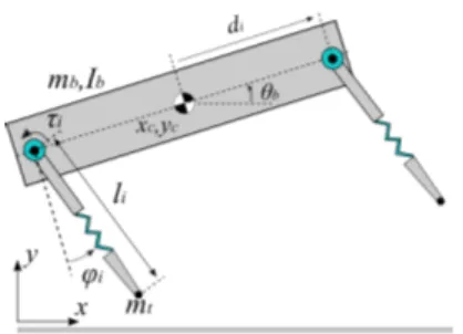
Fig. 1. Planar quadruped model with a stiff body.
Due to the limited attention given to spinal actuation in the robotics literature, there is no single, widely accepted math-ematical model to serve as a basis for studying locomotion within such a morphology. In contrast, the rigid quadruped model that we will use for our comparative study, shown in Fig. 1, has previously been used in the literature. This rigid model consists of a single rigid body with mass mb
and inertiaIb, located at(xC, yC) at an angle of θb with the
2011 IEEE International Conference on Robotics and Automation Shanghai International Conference Center
horizontal. Two legs with compliance k and damping b are attached to the body at distancesdi away from its center of
mass, individually actuated with a torque τi relative to the
body. Each leg can either be in stance or flight, with the leg angle relative to the body vertical denoted with ϕi and its
length withli.
βs
φi θbi
τi
Fig. 2. Planar quadruped model with an actuated spinal joint.
In contrast, the new bounding model introduced in this paper is illustrated in Fig. 2 and incorporates an actuated spinal joint connecting two rigid bodies with massesmbi and
inertiasIbi at a horizontal distancedsi from their respective
centers of mass. This spinal joint is assumed to be actuated with a controllable torque τs. We also denote the angle
between the two segments of the robot body withβs.
In the rest of the paper, we will use the subscriptsf and b to replace i in the definitions above and refer to front and back legs and individual body segments, respectively. We have implemented both models using the Working Model 2D environment, which supports numerical simulation of two dimensional rigid-body systems. Since this simulation environment implicitly computes and solves the equations of motion for these models, we do not present detailed deriva-tions of the associated dynamics in this paper. Further details and specific parameters for the simulation environment we use for our results are given in Section IV-A.
III. CONTROL OFQUADRUPEDALBOUNDING
In this section, we describe bounding controllers for both the stiff-backed and the new jointed-spine quadruped models, consisting of high-level state machines that modulate com-mands to the actuated degrees of freedom, which are then tracked by local PID controllers. We assume leg touchdown and liftoff events can be detected to trigger state transitions. The only other sensors in both systems are assumed to be encoders on hip joints and the body joint to measure their relative angles and support local PID control laws.
A. Bounding with a Stiff Spine TABLE I
HIGH-LEVEL STATE MACHINE FOR STIFF-BACKED BOUNDING. State Target Angles Trigger Event Double Flight (ϕbtd, ϕftd) Back leg lift-off
Front Leg Stance (ϕbtd, ϕflo) Front leg touchdown
Double Stance (ϕblo, ϕflo) Back leg touchdown Back Leg Stance (ϕblo, ϕftd) Front leg lift-off
The bounding gait controller we use for the stiff backed robot model has the same structure with the controllers used
in previous research focused on stiff quadrupedal bounding [7, 8, 21], consisting of a reactive state machine that responds to leg contact events. The desired bounding behavior pro-ceeds through four different states as shown in Table I. The last column in this table indicates the event that leads into the state, whereas the middle column indicates target angles for both the front and back legs that are activated when the corresponding state is entered. Combined with the gains for the local PID controllers, the resulting behavior can hence be represented by the vector
psb:= [ϕbtd, ϕblo, ˙ϕb, ϕftd, ϕflo, ˙ϕf, Kp, Ki, Kd] T
(1) whereKp,Ki andKd denote local PID gains to track linear
leg and body joint reference trajectories. B. Bounding with a Jointed Spine
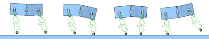
Bounding with an actuated spine requires the control of the spinal joint. Consequently, we augment the high-level state machine for stiff-backed bounding described in Section III-A with additional semantics, resulting in the state machine illustrated in Fig. 3. Our extensions are loosely inspired from biomechanics literature on quadrupedal bounding observed in legged vertebrates [1, 3, 28], cheetahs in particular.
Fig. 3. High-level state machine for bounding with an actuated spinal joint. Each state illustrates how the robot body and legs are expected to be configured. Transitions indicate associated leg contact events.
The key observation in this context is that the spinal joint has two dominant configurations: convex and concave. The former increases stride length by increasing touchdown angles for both legs while the latter prepares the kinematics for additional thrust from the spinal actuator. The following paragraphs present descriptions of each of these states.
1) Double Flight: This state starts with the back leg lifting off during the back leg stance phase. Both legs are then commanded to go to pre-specified touchdown angles ϕbtd
andϕftd. The robot body assumes a convex shape with an
angleβcx, increasing the stride length for the following step.
2) Front Leg Stance: This state starts with the front leg touching the ground during the double flight phase. The spine actuator then assumes a concave shape with an angle βcv,
helping increase the stride length of the back leg. In this state, the front leg maintains backwards motion with a sweep limit, while the back leg maintains its touchdown angle in flight.
3) Double Leg Stance: This state starts with the back leg touching the ground during the front leg stance phase. Following this transition, the front leg spring quickly starts compressing and the back leg starts to shorten in length. Both legs are commanded to go to their liftoff anglesϕbloandϕflo
at predefined speedsϕ˙b andϕ˙f. The spine actuator is used
to maintain a concave body shape to ensure and prepare for supplying additional power during front leg retraction.
4) Back Leg Stance: This state starts with the front leg lifting off the ground during the double leg stance phase. The spine actuator then forms a convex shape, while the back leg maintains its liftoff angle and experiences maximum compression. On the other hand, the front leg actuator is commanded to go towards its touchdown angle position.
Given these four phases, the bounding controller with the flexible body joint is represented with the parameter vector
pf b := [ϕbtd, ϕblo, ˙ϕb, ϕftd, ϕflo, ˙ϕf, βcx, βcv, ˙βs,
Kp, Ki, Kd, Kps, Kis, Kds]T (2)
where Kp, Ki and Kd denote local PID controller gains
whereas angle parameters and their velocities parametrize linear trajectories for the body and leg angles starting from their current position towards their target angles.
C. Local PID Controllers
In all high level controller states for bounding with both the stiff and jointed back morphologies, local PID controllers are used for each actuator to determine associated torque commands. Torque commands for legs in both models and the body joint are computed as
τj= Kpej(t) + Kj Z t 0 ej(t)dt + Kd dej(t) dt , (3)
withj indexes either the leg number or the body joint. Leg and body tracking errors are respectively defined asei(t) :=
ϕ∗
i(t) − ϕi(t), and eb(t) := βs∗(t) − βs(t).
The desired angles for both the legs and the spine are determined by the current phase of the high-level controller and the controller parameters in psb and pf b for the
stiff-backed and flexible-spine models, respectively. For both models, the computation of the desired angles for the legs depend on whether they are individually in stance or flight. During stance, we have
ϕ∗ i(t) = ( ϕi(ttd) + ˙ϕi(t − ttd) ift − ttd< ϕilo−ϕitd ˙ ϕi ϕilo otherwise .
Similarly, during flight, we have ϕ∗ i(t) = ( ϕi(tlo) − ˙ϕi(t − tlo) if t − tlo< ϕitd−ϕilo ˙ ϕi ϕitd otherwise .
The spine actuator is controlled in a similar fashion with its concave and convex poses using the target angles determined by the parameter vector in (2).
IV. SIMULATIONRESULTS
In this section, we present a comparison of the “best” gait performances for the stiff and jointed back bounding controllers, obtained through an optimization framework to automatically tune gait parameters, resulting in a fair characterization of performance in terms of speed, stability and efficiency for both models.
A. Simulation Environment
We have implemented both models described in Section II in the Working Model 2D environment which supports numerical simulation of articulated rigid-body systems with collisions and models of surface interaction. In order to implement the stiff-backed model, we rigidly locked the body joint of the flexible model, keeping all other system parameters identical. All simulations were run with a small, constant time step of10−3s in order to ensure numerical
ac-curacy of the results. Table II details kinematic and dynamic parameters we have chosen for our models, mirroring the morphology of a cheetah as much as possible except perhaps leg compliance and damping constants [28]. Note that we use the same total body mass for both models in order to ensure a fair comparison of performance even though the spinal motor is likely to increase the total mass of the jointed model. In practice, this choice may be justified by choosing a smaller payload capacity for the jointed robot.
TABLE II
SYSTEM PARAMETERS FOR BOTH BOUNDING MODELS. Param. Value Param. Value
mbi 10kg mb 20kg Ibi 1.3kg-m2 Ib 3.85kg-m2 di 0.365m dsi 0.25m k 3500N/m b 55N m/s l 0.8m τmax 200N m µs 0.9 µk 0.8 i ∈ {f, b}, f : front, b: back µs,µk: Static and kinetic friction
Given a set of controller parameters, simulations were started from an initial condition with a forward speed of 1m/s and a height of 0.75 m and executed for 32s. System trajectories were then transferred to Matlab for stability analysis and visualization. A simulation run was considered stable if the system trajectories converged to a limit-cycle in the steady-state. This was verified using the difference in system states from one touchdown of the front leg to the next with a tolerance of 10−1 on the norm of the error.
For each successful run, we compute a performance measure that is inspired from the commonly used specific resistance [29], modified to slightly favor speed over efficiency with ǫ := P/mgv3
, where P denotes the average of either instantaneous power or its absolute value andv denotes the average velocity across the last five steady-state strides. B. Nelder-Mead Optimization
Nelder-Mead is an efficient, simplex-based numerical opti-mization method [30] that approximates gradient descent but
requires much fewer evaluations of the objective function. Consequently, it is suitable for robotic applications where the evaluation of the objective function requires running experiments with a physical robot [23], or simulations that may take a long time to complete. Since our automated tuning of the bounding controllers rely on running a rather slow simulation for 32s in simulation time, we will use the Nelder-Mead framework to find controller parameters that minimize ǫ. 2 4 6 8 0 0.1 0.2 0.3 0.4 0.5 Number of turns
Cost function value
Stopping Cost 2 4 6 8 0 0.02 0.04 0.06 0.08 0.1 Number of turns
Cost function value
Fig. 4. Progression of the Nelder-Mead optimization for stiff backed (left) and actuated spine (right) models. Red squares plot the stopping criteria functionC, whereas blue stars represent the best vertex cost values for each simplex. Each “turn” corresponds to five Nelder-Mead iterations.
For the stiff-backed bounding model, we use the parameter set defined in (1) that corresponds to aD = 9 dimensional space of independent variables for optimization. In contrast, for the model with a jointed spine, we use the parameter set defined in (2) that corresponds to a D = 15 dimensional space. In both cases, we start the optimization from a manu-ally tuned initial condition that realizes the desired high-level state transition sequence and a gait with reasonable stability. We then run the Nelder-Mead algorithm until convergence, defined through a stopping function estimating the size of the current simplex asC =pP
i(ǫi− ¯ǫ)2/(D + 1), where ǫi denotes the objective function value for different vertices.
When this function falls below a certain threshold (10−3
in our case), the optimization is terminated and is assumed to be converged. Fig. 4 illustrates the progressions of both the objective function and the stopping criteria function for both models. Parameter sets obtained at the end of these optimizations are given in Tables III and IV.
TABLE III
OPTIMAL GAIT PARAMETER FORSTIFFBACKEDBOUNDING
Parameter Value Kp, Ki, Kd (338.2, 0.08, 6.7) ϕtdf, ϕlof, ˙ϕf (0.4rad, -0.03 rad, 4.25 rad/s)
ϕtdb, ϕlob, ˙ϕb (0.27rad, -0.11 rad, 4.5 rad/s)
TABLE IV
OPTIMAL GAIT PARAMETERS FORACTUATEDSPINEBOUNDING
Parameter Value Kp, Ki, Kd (524.7, 0.11, 6.9) Kps, Kis, Kds (1737, 0.03, 330.3) ϕtdf, ϕlof, ˙ϕf (0.3rad, 0.17 rad, 3.43 rad/s)
ϕtdb, ϕlob, ˙ϕb (0.3rad, -0.12 rad, 4.93 rad/s)
βcx, βcv, ˙βs (0.1rad, -0.22 rad, 23.05 rad/s) C. Simulation Results for Bounding with a Stiff Spine
Optimal control parameters for the stiff-backed bounding model result in the behavior illustrated in the snapshots of
Fig. 5. Snapshots of optimal bounding with the stiff-backed model.
0.735 0.74 0.745 0.75 0.755 COM Height (m) 1.6 1.8 2 Speed (m/s) Time (s) Foot Height (m) 30.5 31 31.5 32 0 0.02 0.04 Back Front
Fig. 6. Body height (top), horizontal velocity (middle) and foot clearance (bottom) trajectories for bounding with the stiff-backed model. Green dashed lines in the top two plots indicate the average horizontal speed and heights. Shaded regions in the bottom indicate different controller phases.
Fig. 5. Body height and forward speed trajectories associated with this gait are shown in Fig. 6. With these parameters, stiff-backed bounding reached an average running speed of 1.75m/s and a maximum body height of approximately 0.76m. The robot has a small but distinct flight phase with a maximum foot clearance of up to 0.035m as shown in Fig. 6.
0 200 400 Power (W) 30.5 31 31.5 32 −100 −50 0 50 100 Time (s) Torque (Nm) Front Back
Fig. 7. Power consumption (top) and torque output (bottom) of motors. Blue dotted line represents front hip motor and black line back hip motor.
TABLE V
SPECIFIC RESISTANCE VALUES FOR BOUNDING BEHAVIORS. Model ǫ with Avg. Power ǫ with Avg. Abs. Power
stiff 0.127 0.309
jointed total 0.227 0.755
jointed legs 0.024 0.371
In order to achieve the bounding gait, both hip motors individually consume less than 400W each instantaneously with averages being much lower. Fig. 7 also shows that both motors output less than 90N m torque on the legs. Based on these figures, the specific resistance of the robot during steady-state bounding is given in Table V, where values
obtained from the average of both instantaneous power and its absolute value are given. The optimization was done with the average absolute power, but the direct average of the power is included to give a sense of how passive compliance would benefit performance.
D. Simulation Results for Bounding with an Actuated Spine
Fig. 8. Snapshots of optimal bounding with the actuated spine model.
Similar to our simulations with the stiff-backed bounding model, Fig. 8 illustrates snapshots from steady-state bound-ing with the actuated spine model. The video extension accompanying this paper also shows both real-time and slow motion versions of optimal bounding with this model using the parameters of Table IV. These experiments demonstrate the validity of our controller since both the bending direc-tions of the body and the progression of leg contact states are consistent with the proposed high-level state machine.
0.72 0.74 0.76 0.78 COM Height (m) 1.9 2 2.1 2.2 Speed (m/s) Time (s) Foot Height (m) 30.50 31 31.5 32 0.05 0.1 0.15 Back Front
Fig. 9. Body height (top), horizontal velocity (middle) and foot clearance (bottom) trajectories for bounding with the actuated spine model. Green dashed lines in the top two plots indicate the average horizontal speed and heights. Shaded regions in the bottom indicate different controller phases.
−500 0 500 1000 Power (W) 30.5 31 31.5 32 −200 −100 0 100 200 Time (s) Torque (Nm) Spine Front Back
Fig. 10. Power consumption (top) and torque outputs (bottom) of motors. Red dashed line represents spine motor, blue dotted line front hip motor and black line back hip motor.
As shown in Fig. 9, the actuated spine model achieves a stable bounding gait with an average horizontal speed of
2m/s. As shown in Fig. 9, the hopping height of the robot fluctuates between 0.7m and 0.8m, with the corresponding leg clearances illustrated in Fig. 9. Not surprisingly, the body joint experiences higher loads than the leg actuators, with a maximum instantaneous power of 1200W but a much lower average. Fig. 10 also shows that spine motor torque saturates during the front leg stance. Bounding with the actuated spine model yields specific resistance values shown in Table V. E. Discussion
The most important outcome of our results is the observa-tion that the actuated spinal joint allows bounding at higher speeds. Consistent with studies of how increases in speed are obtained by quadrupedal animals in the biomechanics liter-ature [10], this increase in speed is primarily a consequence of the increase in stride length as illustrated by Fig. 11. The average stride lengths for the stiff and flexible spine models are 0.58m and 0.86m, respectively. Interestingly, if Figures 6 and 9 are studied carefully, one can notice that the stride frequency for the optimal bounding gait with the flexible spine model is in fact smaller, corresponding to a slowing down of the stepping frequency. This means that the increase in stride length through the use of the spinal joint is not only sufficient to compensate for the slowing down in the stride frequency, but also allows an overall increase in the average speed from 1.75m/s to 2.02m/s. 1 2 3 4 5 6 0.6 0.7 0.8 Stride number Stride length (m) Rear Legs 1 2 3 4 5 6 0.6 0.7 0.8 Stride number Stride length (m) Front Legs Rigid Spine Jointed Spine
Fig. 11. Stride lengths for the back (left plot) and front (right plot) legs for the last six bounding steps. Red stars illustrate stride lengths for the actuated spine model whereas the blue squares correspond to the stiff backed model.
Some additional insight into the bounding behavior may be gained by inspection of the optimal parameters obtained for the actuated spine model. In particular, the back leg is commanded at a higher velocity (4.93rad/s) following touchdown even though its range of travel is diminished (0.42rad) compared to the front leg (0.47rad). This trans-lates into the back leg exerting larger torques during stance, also confirmed by the torque profiles of Fig. 10. This would motivate stronger actuators for the back legs of a possible physical realization of this gait, which is also intuitively con-sistent with what we observe in most quadrupedal runners.
When the specific resistance values are compared, a number of interesting features emerge. First of all, there is a substantial difference between specific resistance values computed with the averages of instantaneous power and its absolute value. This suggests that both the leg motors and particularly the body joint do significant negative work and would substantially benefit from some form of passive compliance. This is both intuitive and consistent with ex-isting conclusions on how springs can improve efficiency
of locomotion. Naturally, when such passively compliant elements are incorporated into the system, control strategies need to be adapted accordingly. Finally, we can also see that when only the legs are considered for both models using the absolute value of the power for averaging, both bounding models have similar specific resistance values with 0.309 for the stiff and 0.371 for the jointed back models. This shows that the incorporation of the jointed back does not substantially change the power budget of leg actuators.
V. CONCLUSION ANDFUTUREWORK
In this paper we have introduced a new quadruped robot model with an actuated spinal joint. Inspired from the morphology of fast running land mammals, we have designed a new bounding gait controller that works with our new model. We compared our model with a commonly used rigid bounding model through corresponding optimized bounding gaits and showed the effects of an actuated spine mechanism on the running speed and hopping height.
Our simulation experiments show that the actuated spine mechanism helps increase stride length, resulting in in-creased horizontal speed. The actuated spine is also capable of achieving higher hopping heights of the robot body, which helps the bounding behavior overcome bigger obstacles, con-sistent with its use by quadrupedal animals. The efficiency of the new bounding behavior was found to be not unreasonably different from stiff-backed bounding even with the additional actuator on the body joint.
In the near future, we will investigate using passively compliant elements both for the body joint and the legs to eliminate inefficiencies arising from negative work. This would also address practical problems such as controller bandwidth and required motor size towards a realistic im-plementation of the bounding behavior with jointed spine. Another important direction is to investigate how the front and back legs should be differentiated to motivate more efficient distribution of the power budget on a physical robot platform. In any case, we have been able to demonstrate in this paper that the incorporation of a flexible spine may be advantageous in improving quadrupedal gait performance.
VI. ACKNOWLEDGMENTS
This work was supported by TUBITAK, through project 109E032 and Utku C¸ ulha’s scholarship.
REFERENCES
[1] P. P. Gambaryan, How Mammals Run: Anatomical Adaptations. Wi-ley, 1974.
[2] C. R. Taylor, N. C. Heglund, and G. M. O. Maloiy, “Energetics and mechanics of terrestrial locomotion,” J. of Experimental Biology, vol. 97, pp. 1–21, 1982.
[3] T. M. Caro, “Ungulate antipredator behaviour: Preliminary and com-parative data from african bovids,” Behavior, vol. 128, no. 3-4, pp. 189–228, 1994.
[4] M. H. Raibert, Legged robots that balance. Cambridge, MA, USA: MIT Press, 1986.
[5] ——, “Trotting, pacing and bounding by a quadruped robot,” J. of
Biomechanics, vol. 23, no. 1, pp. 79–98, 1990.
[6] J. Estremera and K. J. Waldron, “Thrust control, stabilization and energetics of a quadruped running robot,” Int. Journal of Robotics
Research, vol. 27, pp. 1135–1151, 2008.
[7] I. Poulakakis and J. A. Smith, “Modeling and experiments of unteth-ered quadrupedal running with a bounding gait: The Scout II robot,”
Int. Journal of Robotics Research, vol. 24, pp. 239–256, 2005.
[8] J. A. Smith, I. Sharf, and M. Trentini, “Bounding gait in a hybrid wheeled-leg robot,” in Proc. of the Int. Conf. on Intelligent Robots
and Systems, 2006.
[9] R. Playter, M. Buehler, and M. Raibert, “BigDog,” in Soc. of
Photo-Optical Instr. Eng. (SPIE) Conf. Series, vol. 6230, Jun. 2006.
[10] L. D. Maes, M. Herbin, R. Hackert, V. L. Bels, and A. Abourachid, “Steady locomotion in dogs: Temporal and associated spatial coordi-nation patterns and the effect of speed,” J. of Experimental Biology, vol. 211, pp. 138–149, 2008.
[11] B. Boszczyk, A. Boszczyk, and R. Putz, “Comparative and functional anatomy of the mammalian lumbar spine,” Anatomical Record, vol. 264, no. 2, pp. 157–168, OCT 1 2001.
[12] K. F. Leeser, “Locomotion experiments on a planar quadruped robot with articulated back spine,” Master’s thesis, Massachusetts Institute of Technology, 1996.
[13] M. F. Silva and J. T. Machado, “A historical perspective of legged robots,” J. of Vibration and Control, vol. 13, pp. 1447–1486, 2007. [14] F. Iida and R. Pfeifer, “Cheap, rapid locomotion of a quadruped robot:
Self-stabilization of bounding gait,” Intelligent Autonomous Systems, vol. 8, pp. 642–649, 2004.
[15] P. Doan, H. D. Vo, H. K. Kim, and S. B. Kim, “A new approach for development of quadruped robot based on biological concepts,” Int. J.
of Precision Eng. and Manifacturing, vol. 11, pp. 559–268, 2010.
[16] D. Campbell and M. Buehler, “Preliminary bounding experiments in a dynamic hexapod,” in Experimental Robotics VIII, B. Siciliano and P. Dario, Eds. Springer-Verlag, 2003, pp. 612–621.
[17] U. Saranli, M. Buehler, and D. E. Koditschek, “RHex: A simple and highly mobile robot,” Int. Journal of Robotics Research, vol. 20, no. 7, pp. 616–631, July 2001.
[18] J. G. Cham, S. A. Bailey, J. E. Clark, R. J. Full, and M. R. Cutkosky, “Fast and robust: Hexapedal robots via shape deposition manufacturing,” Int. Journal of Robotics Research, vol. 21, pp. 869– 883, 2002.
[19] J. M. Morrey, B. Lambrecht, A. D. Horchler, R. E. Ritzmann, and R. D. Quinn, “Highly mobile and robust small quadruped robots,” in
Proc. of the Int. Conf. on Intelligent Robots and Systems, 2003.
[20] S. Kim, J. E. Clark, and M. R. Cutkosky, “iSprawl: Design and tuning for high-speed autonomous open-loop running,” Int. Journal
of Robotics Research, vol. 25, pp. 903–912, 2006.
[21] P. Chatzakos and E. Papadopoulos, “Bio-inspired design of electrically-driven bounding quadrupeds via parametric analysis,”
Mechanism and Machine Theory, vol. 44, no. 3, pp. 559 – 579, 2009,
special Issue on Bio-Inspired Mechanism Engineering.
[22] H. Zou and J. Schmiedeler, “The effect of asymmetrical body-mass distribution on the stability and dynamics of quadruped bounding,”
IEEE Trans. on Robotics, vol. 22, no. 4, pp. 711–723, Aug. 2006.
[23] J. D. Weingarten, G. A. D. Lopes, M. Buehler, R. E. Groff, and D. E. Koditschek, “Automated gait adaptation for legged robots,” in Proc.
of the Int. Conf. on Robotics and Automation, vol. 3, 2004, pp. 2153–
2158.
[24] Z. G. Zhang, H. Kimura, and Y. Fukuoka, “Self-stabilizing dynamics for a quadruped robot and extension toward running on rough terrain,”
J. of Robotics and Mechatronics, vol. 19, no. 1, pp. 3–12, 2007.
[25] J. Buchli and A. J. Ijspeert, “Self-organized adaptive legged locomo-tion in a compliant quadruped robot,” Autonomous Robots, vol. 25, no. 4, pp. 331–347, 2008.
[26] I. Poulakakis, E. Papadopoulos, and M. Buehler, “On the stable passive dynamics of quadrupedal running,” in Proc. of the Int. Conf. on
Robotics and Automation, vol. 1, Sept. 2003, pp. 1368–1373 vol.1.
[27] K. J. Waldron, J. Estremera, P. J. Csonka, and S. P. N. Singh, “Analyz-ing bound“Analyz-ing and gallop“Analyz-ing us“Analyz-ing simple models,” J. of Mechanisms
and Robotics, vol. 1, no. 1, p. 011002, 2009.
[28] L. M. Day and B. C. Jayne, “Interspecific scaling of the morphology and posture of the limbs during the locomotion of cats (felidae),” J.
of Experimental Biology, vol. 210, pp. 642–654, 2007.
[29] G. Gabrielli and T. H. von Karman, “What price speed?” Mechanical
Engineering, vol. 72, no. 10, pp. 775–781, 1950.
[30] J. A. Nelder and R. Mead, “A Simplex Method for Function Mini-mization,” The Computer Journal, vol. 7, no. 4, pp. 308–313, 1965.