/33
'' * « r \ é « í_ j ^· i , -- · '-- ■- _ > у ~·^ -Г^ ¿r" !¿:uí i. ѴІЦ V>' äö: « г ч іё ік ’Т> » « !V iS iíc S ¿ 'r /
'. ξ - ^ »ÿROBUST REGRESSION AND APPLICATIONS
A THESIS PRESENTED BY ARZDAR KIRACI TO
THE INSHTUTE OF
ECONOMICS AND SOCIAL SCIENCES IN PARTIAL FULFILLMENT OF THE
REQUIRMENTS
FOR THE DEGREE OF MASTER OF ECONOMICS
BILKENT UNTVERSTY SEPTEMBER, 1996
A r^bcLxr X iTiXC^
^aiey^nc/af!
H5,
и з
■
[ certitV that I have read this thesis and in my opinion it is fully adequate, in scope and in quality, as a thesis for the degreee o f Master of Economics.
Prof. Dr. .M adZaman
Tj
I certify that I have read this thesis and in my opinion it is fully adequate, in scope and in quality, as a thesis for the degreee o f Master of Economics.
I certify that I have read this thesis and in my opinion it is fully adequate, in scope and in quality, as a thesis for the degreee o f Master of Economics.
Assis. Prof. Dr. ¡Bahri Yılmaz
Approved by the Institude o f Economics and Social Sciences
I certify that I have read this thesis and in my opinion it is fully adequate, in scope and in quality, as a thesis for the degreee o f Master o f Economics.
Prof. Dr. .Asad Zaman
I certify that I have read this thesis and in my opinion it is fully adequate, in scope and in quality, as a thesis for the degreee o f Master o f Economics.
Assoc. Prof. Dr. Syed Mahmud
I certify that I have read this thesis and in my opinion it is fully adequate, in scope and in quality, as a thesis for the degreee of Master o f Economics.
Assis. Prof. Dr. Bahri Yılmaz
Approved by the Institude o f Economics and Social Sciences
Director:
ABSTRACT
ROBUST REGRESSION AND APPLICATIONS
ARZDARKIRACI
M A in Economics
Supervisor: Prof. Dr. Asad Zaman
September 1996
This study analyzes the effect o f outliers in the regression analysis with the help o f a written program in the programing language o f GAUSS. The analysis relies on the subject o f Robust Regression, which is explained and supported by experiments and applications. The applications contain examples to show the superiority o f this technique.
Key Words: Robust Regression, Outlier, Leverage Point, Robust Distance, Least Median Squares, LMS, Least Trinuned Squares, LTS, Minimum Volume Ellipsoid, MVE, Minimum Covariance Determinant, MCD, Program for Robust Regression, Defect o f Ordinary Least Squares Regression.
ÖZET
GÜÇLÜ REGRESYON VE UYGULAMALARI
ARZDAR KIRACI
Yüksek Lisans Tezi, İktisat Bölümü
Tez Yöneticisi: Prof. Dr. Asad Zaman
Eylül 1996
Bu çalışma GAUSS programlama dilinde yazılmış bir programla regresyonda yanlış etki gösteren noktalan incelemektedir. Güçlü Regresyon tekniği açıklanmakta, deneyler ve örneklerle desteklenmektedir. Örnekler Güçlü Regresyonun üstünlüklerim göstermektedir.
Anahtar Kelimeler: Güçlü Regresyon, Uzak Nokta, Etkili Nokta, Güçlü Mesafe, Medyan Kare Minİmizasyonu, LMS, Belirli Toplam Kare Minimizasyonu, LTS, Elipsoid Hacmi Minimizasyonu, MVE, Kovaryans Determinantı Minimizasyonu, MCD, Güçlü Regresyon Programı, Regresyon Hatalan
Acknowledgements
I would like to express my gratitude to Prof Dr. Asad Zaman for his valuable courses in Statistics and Econometrics. I would also thank to Assoc. P ro f Dr. Syed Mahmud and Assis. P ro f Dr. Bahri Yılmaz for their valuable comments..
Contents
1. Introduction
2. R obust Regression
2.1 Outliers and OLS... 4
2
1.1 Sensitivity of OLS.
...5
2.2 Least Median Squares, LMS...6
2.3 Least Trimmed Squares, LTS... 8
2.4 Minimum Volume Ellipsoid, MVE and Minimum Covariance Determinant, MCD... 8
2.5 Famous Example... 10
3. T he P ro g ram Robust 12 3.1 A Guide to The Program Robust... 12
3.2 Algoritms used in Robust... 18
3.2.1 Exact Algoritm.
...18
3.2.1 Random Algoritm
...19
3.3 Effectiveness... 22
4. A pplications 25 4.1 Urban Unincorporated Places...25
4.1.1 Extreme Case
...25
4.1.2 More Data.
...27
4.2 M edium Income and Population in US cities... 28
4.3 Latitude versus Temperature... 42
4.4 Education and Income...42
5. Conclusions 50
6. References
51
7. Appendix
52
1. Introduction
The Ordinary Least Squares Regression (OLS) is the oldest and very easily applicable type of regression. A person familiar with matrix algebra or a scientific calculator, can get the results in a very short time. The results are reliable and counted as admissible until the discovery o f the Bayesian Estimators.
The results o f the OLS are reliable, if the data are also reliable. If there is a possibility o f corrupted data or wrong recordings, blind application o f the OLS leads to very different results. This is due to the fact that OLS is a very equalitarian type o f mathematic process. Every data has to be counted in the regression with its tendencies.
It is shovm that even one corrupted data leads to conflicting and possible opposite results. For example it may show a variable as significant while it is not or makes a variable become dropped. This comes from the fact that OLS tries to minimize the residuals o f all the points, as a result, a data far away from all the other data points tendency increases the residuals o f all the other points.
If we could make a metaphor, if the residuals represent the desire o f food o f the persons in a society, then each would have different desire. It is sometimes the case that, although the biological organism does not need to be fed always, people eat much more than their need. Assuming that there is an outlier person in such a small society, and also assume that people are trying to apply the equalitarian OLS idea.
If for most o f the people the desire for food is just their biological need, than OLS idea would make them loose weight while the outlier fad person would gain kilos. However, if they say that we believe in OLS but after a Robust reasoning, and if they apply this idea, then the outlier would be forced to loose the excess kilos, which is in fact more equalitarian, because it does not harm everybody.
As a result, blind application o f OLS may lead to harmful results. Therefore, it is suitable to go through the concept o f the effects o f corrupted data on OLS.
Robust Regression can be explained as the a technique to identify the data which do not conform to the tendency o f the majority o f observations. It is a natural result that after identifying such data’s it is logical to cancel their effects. In order t make the Robust Regression analysis easier, I have written a program in GAUSS using the tools that can be used in this kind of regression. It identifies the points, which change the results in their absence.
The thesis contains the explanation o f the written program ROBUST, experimented data and results drawn out o f these experiments and applications. The applications contain the illustration o f the superiority o f the Robust Technique used.
2. Robust Regression
2.1 Outliers and OLS
In the literature we have standard assumptions and we can state the robustness o f an estimator to how well the estimator works under failures o f the standard assumptions. The most important assumption is the normality assumption. Normality is important because o f the central limit theorem and computational easiness. The central limit theorem suggest that many random variables may be reasonably well approximated by normal distribution. The second and more important fact is that computational procedures with normal distributions are easy to carry o u t'.
Theoretical and technical developments have introduced new techniques, which doesn’t require the normality. In addition, easiness o f the normality is replaced by computer power. New computers have made possible to shorten the calculation time and even introduced techniques to simulate the computations" by regenerating some variables. The robust procedures are the result o f these developments. Sometimes calculations require exact normality, the lack of this requirement leads to very different results, even when they are close to normal. Robust procedures do not require normality and therefore are superior to the classical procedures^. *
* VVe could have also used the absolute value instead of the square term, and then minimized the sum o f absolute residuals. However, minimizing the sum o f squared residuals is substantially easier.
^ Bootstrapping or generating random numbers with help of computer.
2.1.1 Sensitivity of OLS
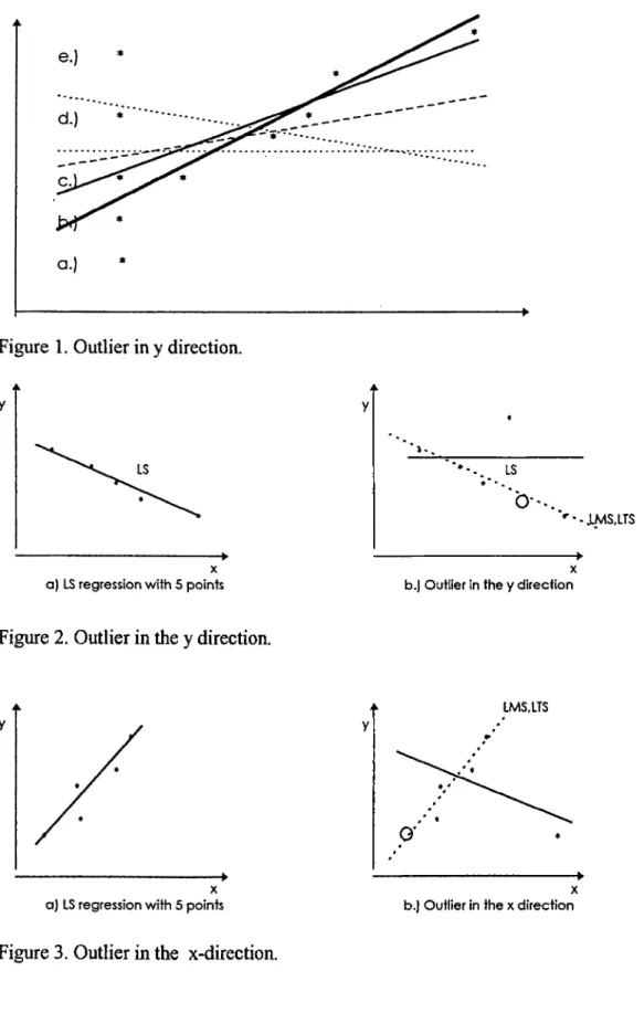
In figure 1 we can see how sensitive the OLS (Ordinary Least squares) estimator is for a regression o f the type y=P)X+Po in case o f bad data or an outliers'* * *. The bold line shows the actual trend o f the data in the case that the first point is recorded correctly (case a). In the other cases, as the point deviates from the actual position the estimator gets worse. Therefore, the OLS is very sensitive to corrupted data.
If we define the i*** residual as r /( p ) =
{y, -
x;P)^ then the LS regression would try tominimize the sum o f squared residuals, which is : S .
In figure^ 1 we see the rotation o f the LS line when the residual o f the first point gets bigger and bigger. OLS tries to minimize the total sum o f squares and in this case the first point adds a very large number to the sum. So it has to be minimized more than the others. As a result, the true tendency cannot be selected in this case.
In figures^ 2 and 3 we have the same situation. In figure 2.a.) we have a negative relation between x and y, however, in 2.b.) it seems to be that there is no relation between x and y. In all o f the figures 2,3 and 4 we see points which are very far apart from the point cloud and therefore they named as
leverage
point.As explained above, the influence o f the leverage points is obvious and it is not always the case that they have a negative effect. In the first three figures they add a large amoimt to the sum o f residuals, increase the variance and show wrong results. However, in figure^ 4 the leverage point is in accordance with the observations and the tendencies. This point is a justification to the tendency o f the data and therefore may determine the value o f R^. We can see from figure 5, that in case a.) the points decreases the value o f to a lower degree with
'* Outliers is a special kind of data, which does not show the general trend o f the other observations.. ’ Appendix page i
* Appendix page i ^ Appendix page ii
wrong direction compared to the dashed tendency. In b.) part it increases to a higher degree and shows a relation where in fact there is none.
Given that OLS is extremely sensitive to outliers and abredant data, a natural way to continue is to identify this sensitivity. The main idea is to delete one or several observations and study the impact on various aspects o f the regression. When one observation is deleted, all o f the regression statistics change, but we should keep in mind that if there are wrong observations in the data set these statistics are in fact wrong. A number o f methods have been proposed to asses the impact o f dropping an observation on various regression statistics.
The intended objective o f sensitivity analysis is to asses whether the OLS regression results are seriously affected by the presence o f a small group o f observations. While sensitivity measures taken in combination can, in hands o f experts, achieve this objective, there now exist simple ways, which can routinely identify the extend to which OLS is affected by outlying subgroups of observations. These include the high breakdown regression estimators, including LMS^, LTS’ ,MVE“^ and MCD* **‘ . Application o f these techniques immediately reveals the presence of subgroups o f observations that differ substantially from the other points or exert undue influence on, the regression results. The written program named R obust uses this tools to identify the outliers, which are explained in a while.
2.2 Least Median Squares, LMS
Least median squares technique has several properties, which makes it very attractive for the preliminary analysis. In particular, if results from an LMS analysis are similar to OLS, we can safely conclude that no small subgroup o f the data is causing undue distortions o f the OLS results.
The problem with the OLS is that it fails in the case o f even one o f the observation is bad, as we have seen in the previous section. Obviously OLS will fail again if the number o f bad
* Least Median Squares, by Peter J. Rousseew 1984 10Least Trimmed Squares, by Peter J. Rousseew 1984Minimum Volume Elipsoid, by Peter J. Rousseew 1984. ** Minimum Covariance Determinant, by Peter J. Rousseew 1984.
recordings increases. We obviously need to deal v^th larger number o f bad observations. The LMS has the property that it works even when half o f the data is contamined.
If we want to explain the process o f LMS we have to consider some specific residuals. For
any p, let r/( P ) =
(y, -
,r;p)^ be the squared residual at the t-th observation. Rearrange thesesquared residuals in increasing order by defining ri(P) the smallest residual, r2(P) the second
smallest and ri{(P) the k*** in the order o f residuals. The LMS is defined to be the value o f p for which the median o f the squares is the smallest possible. The median is most o f the time the half o f the number o f observations.
If we take the median o f the residuals, we allow some points to have very large residual numbers. This situation avoids cases as in figure 2-5 and it acts as if ignoring the presence o f far apart points.
In the case o f figine I, LMS will give the first data the highest residual and the assigned coefficient b will be as if the first data is not present. In figures 2 and 3 the dashed lines show the result o f the minimization o f the median residual. They are similar to the original LS regression with the correct data. More explanation about this type of regression is in the program algorithm part. As a result we can summarize LMS as:
Minimize med(r^)
p
~ I
In order to minimize the this special number we can consider to take subgroups o f sum fixed number. If we assume that we have 10 observations and 3 variables. We can consider all o f the subgroups o f size 3 made up o f these 10 observations, which makes 120 possibilities. You take one o f these subgroups, draw the best-fit line going through the and consider this line as the regression line and look at the median residual. If this is the smallest among the 120 other median residuals then record the beta or coefficient as the solution o f the LMS coefficient. This process can be used also in the following sections.
2.3 Least Trimmed Squares, LTS
In this regression type the outliers are identified by looking for cases where the sum o f the smaller number o f residuals is preferred. It is more alike to OLS than the LMS. In this case the first half o f the smallest residuals are added together. Again defining ri(P) the smallest residual, r2(P) the second smallest and rk(P) the k*^ in the ordered form from smallest to the
largest, you add up the first h o f them, where h is half o f the data or any number that does not include the corrupted data.
h
As a result, LTS corresponds to minimize: ^
(=1
The difference between LMS and LTS is in the considered number o f points. LMS concentrates only on one point while LTS concentrates on at least half number o f points. So the concept o f efficiency says that both are not as efficient as the OLS, which considers all o f the points. The LTS has at least 50% o f efficiency, while the LMS has 0% . However, if we use this type o f regressions to identify the outliers and then make OLS after the dropped observations then the efficiency increases. In other words, if we delete these outliers and run OLS in the rest (Reweighted OLS), then we have the highest possible efficiency.
Both LMS and LTS are means to detect the minimum possible residuals and so detect the outliers. In order to identify the leverage points, which play the decisive role we need to introduce two more methods.
2.4 Minimum Volume Ellipsoid, MVE and
Minimum Covariance Determinant, MCD
The idea in the MVE is to detect the points that are far away from the rest o f the point crowd. In figure 5 the three points are the leverage points, which are far away from the center o f the crowd.
The classical method to determine the leverage points is the Mahalanobis distance, which has the following form:
n: Number o f observations
1 ”
= (;c, - n X ) ) C { X y \ x , - n X ) ) ‘
7-(A-) = -!.X .x,
C{X)
= -T{X)y{x, - n x ) )
The arithmetic mean
T(X)
is a kind o f measure for the center of the point cloud and the matrixC(X)
a kind o f measure for the variance or spreadness. If a point far away from the center with some factor larger than the spreadness is identified as leverage point by the classical method. The classical method o f leverage point detection suffers from the same reason as the OLS does. It considers all o f the points and in turn the influence o f the outliers also. This may be beneficial for the bad leverage points.With the increasing number o f bad data the spreadness matrix
C(X)
increases and it becomes even harder to identify the points far apart. In figure*^ 6 we can see the 97.5 tolerance ellipsoid that is a special ellipsoid. After that ellipsoid the points are identified as leverage point and are rejected. The big ellipsoid, which is influenced by the three leverage points contains them. The robust distance ellipsoid, however, identifies them.The way to identify the outlying points is in the same way as in the previous two topics, namely, finding a way to discriminate them in forming some subgroups. In MVE you form a subgroup o f some predetermined number o f elements and minimize the a function, which is proportional to the volume they form. This volume should contain at least half o f the elements or the number o f points wanted. At the end the subgroup that has the minimum volume and containing the desired number o f elements is accepted as the base or central group. According to this subgroup
T(X)
andC(X)
are determ ined.,Standartized residuals are formed by dividing the residuals by standard deviation, and usually standartized residuals with large number are accepted as outliers. In this case also we want to identify points far away from the cloud if they have a distance larger than the
square distribution 97.5% and variable times o f freedom. These are the leverage points. Formally, they are far apart if:
(X, - nX) ) C{ X) %x, - n X ) ) ' > zi,.e,o.<rr,
In the case o f MCD, you take all possible combinations o f half number o f data points and try to minimize the covariance matrix
C{X).
In this case also the minimizing subgroup determines the mean and covariance and similar to MVE the points exceeding some value are regarded asleverage
points.In all o f the four robust regression procedures, the process is to look for some subgroups. The idea is that if there is a tendency than this subgroup should have the pure tendency and all others are an accumulation to it. The ones not suited will be seen as outlier or distant point (leverage point).
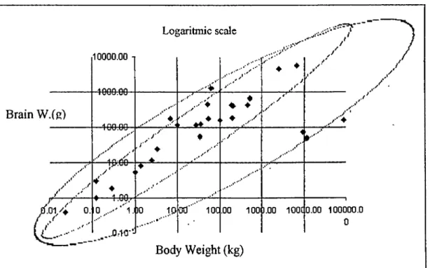
2.5 Famous Example
This is a famous example, because it reflects a real world situation where the facts are
10000.00 -1 A onn no Lo{»aritm ic S( ....¡ c calc .··· * , /·' y' .,*y~ y / . / . B r a i n W . ( g ) 1 uuu.uu A nn nn ■ r ' y ■ ♦ ♦ ♦ t· / y x' ' y' y .' .X' y ·· -in.On . / ·'■ ♦ . ♦ ♦ .t' .. /* ’ i .1*'' 1 y.UU ♦ ▲ A on ♦ ► / ' 0. 10^....''’' l . 30 10 .··*** B o d ; 00’" 100 W e i g h t .00 100I ( k g ) 3.00 100C 0.00 100000.0 0
observable and used by most o f the authors in this concept. T a b l e 1 summarizes the relation between brain-weight o f a species and the body-weight o f it with the previous figure.
In figure*'* 6 and 7 we can see tolerance ellipsoid for the MD and the robust distance. Obviously as in table 1, the classical methods are unable to detect the difference between the recent habitants and the extreme cases, which are the very oldest and very new ones. The MD identifies only one dinosaur as leverage point, while the robust distance identifies all o f the five species that are different from the other points. The results o f OLS are:
F-Value = 40.26061840 Res. SS.= 28.41083006 Std. err= 1.045334508
R2-Value=0.6076100612 Est. SS.= 43.99375337 Case Num= 28
A d j . R2 =0.5925181405 Tot. SS.= 72.40458343 Var. No.= 2
Variable Est.Coe. Confidence Intrv. Str. err T-Value P-Value
Body W. Constant 1.225 ( 0.6880 to 1.762) -0.71659 (-1.8858 to 0.452) 0.19307 0.42037 6.3451 -1.7047 0 . 0 0 0 0 0 0.10018
If we exclude the variables which have a standartized residual larger than 2.5 deviations and change the direction o f the direction against the direction of the trend o f the data and repeat the regression we get the following results:
F-Value = 556.9207362 Res. SS.= 1.710742488 Std. err=0.2854188641
R2-Value=0.9636628370 Est. SS.= 45.36895075 Case Num= 23
Adj. R2 =0.9619324959 Tot. SS.= 47.07969324 Var. No.= 2
Variable Est.Coe. Confidence Intrv. Str. err T-Value P-Value
Body W. Constant 1.2834 ( 1.1292 to 1.4376) 0.05438 -1.0677 (-1.4001 to -0.7352) 0.11721 23.599 -9.1089 1.3387E-16 9.6762E-09
The results suggests that leaving the bad residual points out we get an almost exact relation between these variables. The residual sum o f squares decreases drastically and the standard error makes forecasting four times precise. The R^-value and the F-value increases to show the increase o f precision in the regression. Therefore, if OLS shows a relation between the variables we have to keep in mind the possibility o f figure 2,3 and 5. An outlier may cause to make a positive relation look like negative or show no relation.
Appendix page VÜ Appendix page ii
3. The Program Robust
3.1 A Guide to The Program Robust
I have met no program yet that includes four o f the techniques LMS, LTS, MVE and MCD. Therefore there exists also no program that decides on the
good
orbad leverage
points. I hope to be useful to the ones who use it.The program starts with:
Robust Regression Program
by Arzdar Kiraci Version 1.0
at the top and a help line at the bottom indicating the possible operation or the limits o f the input during the choice. For example we see at the bottom:
Please use the Arrow keys and also Spacebar or ENTER for option change Press any key to continue
During the menu choices you have to use the cursor keys to move the cursor to the choices and press space or ENTER (which do the same job and both are used to accept the choice where the cursor is on). If a choice is made the squared brackets disappear the printing changes to large caps, for example, before choice:
Type of Robust Regression: [Lms] [Lts] [Mve] [Med]
and after pressing space:
Type of Robust Regression: [Lms] [Lts] MVE [Med]
At any time you can move the blanking cursor key to the desired level and change the selection.
There are two main menus, one to make general choices and second to make regression specific choices. The first menu looks like the following:
Type of Robust Regression: Combinations: (Lms) LTS [Randomx .... ] [Mve] EXACT (Med)
Input file name :brainlog.dat
Output name :brainlog.lms
Case number :28
Variable number :
Variable position :
How much output : [Small] [Medium] [Large]
Data plot on : [Non] [Estimated] [Index] [Both]
Outer Diagnostics : [Yes] [No]
[Execute]
Enter variable number in your data set
If we go through the explanation o f each step we can say the followings: For the type of the regression you jum p to the position o f the regression you want to perform and press space, for example if you choose MCD it will appear to be:
Type of Robust Regression: [Lms] [Lts] [Mve] MCD
For the choice o f the replications, you can choose to have all o f the possible combinations or randomly generate some subgroups. If the data set is very large with many variables it may take a very long time to arrive at an exact solution. With a large number o f random generations you will end high probability in an exact solution.
If you are in the position " [ E x a c t ] " press space and make your choice. If you want random generations, you have to enter the number o f replications you want. In this case if your cursor is blanking in the place o f [R an do mx ...] , begin to write the number. If you press a non-number element a beep signal will be heard, requiring you to give the correct number. This will look like as follows:
Combinations: Randomx 1250 [Exact]
In the third position you have to choose the name o f the input file. The file has to be in the same directory as where you run this program. If you write the file name wrong or if it does not exist an error message v^ll appear. As long as the cursor is in the same position you can enter the name, however you have to press Enter or space in order to be accepted. If it is accepted, the name will be written immediatelly. It will look like the following while you are writing:
Input file name :brainl_
After that you have to enter the output file name, with the care that if there exists a file with the same name that it will be erased. Same rules as input file name applies also here. As an example we can consider the main menu above.
In the option "Case number:" you have to enter the observation number. Your data set have to be in row major ordered, that is every row in your data set have to contain one observation. If your data set is not compatible with the information you entered the program will not execute. The main menu is an example for the appearance.
In the option "Variable number:", you have to enter the number o f columns in the data set. It should include all o f the variables, even if there exists an index colomn. In the next stage you can exclude the variables you don't want to have in your analysis.
In the next stage where you enter the position o f the variables include to give the names o f the variables and their positions. I f you press space or enter when you are in this option a screen will appear as follows:
Name Position
Res.Var. 0
ok
You write the name o f the response variable in this box and give its position. By moving the cursor key to the bottom you can finish this section. Again, if you make a wrong input an error message will appear and a new input is desired. After that the following menu will appear: Variables to exclude Name Res.Var. Var 1 Var 2 Exc- Inc-[X] [ ] [X]
Name Exc-
Inc-ok
In this menu you can change at any time the variable name and if you want it to be excluded from the regression you can go to the “Exc-” part and exclude it. At the end you go the “ok” part and press space.
Then you are asked how much the lenght o f your output should be. If you choose small output then your results will be limited with the basic results. The observations are not printed on the output file. If you choose medium output the OLS results are extended. In large the maximum possible output is produced and if you want outlier diagnostics you have to make that choice to see the list o f good and bad leverage points, as in example below:
How much output : [Small] [Medium] LARGE
It also possible to see the distance and residual plots. They use the DOS prompt as output so they are not supported by any graphic option possibility. For the brain weight and body weight example you get the residual plot as the one below:____________
3.25 2.5 -2.5 -3.2 ---11 -11 1 1 — 1 ---11 2
The numbers indicate the number o f points in this range. The horizontal axis is either the index, which is the order o f the data, or it is the order o f the estimated response variable from smaller to the larger one. The same is true for the distance plots. The residual plots are for LMS and LTS, the distance plots are for MVE and MCD. As in the example below if you select “Non” no plot is drawn. If you select “Estimated” the estimated values vs. the residuals are drawn, this case changes to index vs. residual plot if you select the mode “Index”. If you select both, both are dravm. The same output is produced with different locations on the horizontal axis. In example below you can make the index choice.
Data plot on : [Non] [Estimated] i n d e x [Both]
In example below you make the decision to outlier diagnostics. Outlier diagnostics runs as follows: First you run LMS or LTS to provide the necessary residuals for the outlier diagnostics and the run MVE or MCD to get the distances necessary for the last part.
Outer Diagnostics : [Yes] [No]
At the end you move the cursor to the bottom to execute the program. If there are missing or wrong values, the explanation will appear and the correct values are desired. Only after that you can go to the stage below.
[Execute]
In the next stage the following menu appears for LMS,LTS and MVE. The MCD does not the menu because it automatically takes half o f the data to the minimization process. For LMS and LTS we have;
Do you want a constant to be added : YES Give the size of the elementary set: ALL
Which element should be minimized : _
[Execute]
For MVE we have:
Do you want a constant to be added : YES Give the size of the elementary set: ALL Ellipsoid contains how many points : _
[Execute]
[No] [Size:1
[No] (Size:;
If you don’t want to add constant you move the cursor to the right side and press space, by default a constant is added. By moving the cursor to the size part you can select the size o f the elementary subgroup, but a more time consuming choice is the choice o f all elementary subsets starting with the minimum possible and ending with the regression on all the elements At the end selecting the best subgroup that minimizes the target element (LMS) or target sum (LTS). At the last part the size o f the target element is given. While executing the program the following screen will appear:
Cycles left: 1000
Time passed: 1 sec
After going through the calculations the last choice must be made to continue with same data or not. If you select Yes all information must be again entered, but if you choose the old date you ju st have to enter the new regression type, but we don’t have to forget to change the output file name if necessary. At the end the following screen will appear:
Do you want to continue?
YES yes, same data no
3.2 Algoritms used in Robust
3.2.1 Exact Algoritm
The idea in robust regression was to generate subgroups and find the best subgroup that minimizes objective function. The objective function was the median residual in the regression LMS, it was the partial sum o f the smalllest residuals in LTS, it was the volume funciton in MVE and it was the covariance matrix in the MCD.
In the exact algoritm all possible combinations o f the subsamples had to be generated. In order to achieve this goal, two matrices o f the elementary subgroup size are formed. Assuming that there are 15 observationsand the elementary subgroup is o f the size 4, then the two matrices look like the following when initialized.
indxit
= [1 2 3 4] /cr = [12 13 14 15]i
i
The last colomn of the matrix indxit acts as a counter. After getting and ordering the residuals, the objective function is calculated and if it has the minimum it is recorded as best index. In order to get the other subgroup the last colomn is incremented by one. It is incremented till it is equal to the last colomn or the corresponding colomn in the icr matrix. After incrementing the matrix indxit gets the following form.
incLxit = [\
2 4 5]icr = [\2
13 14 15]i
r
Every time the last colomn o f indxit equals to the last colomn o f the matrix icr, the colomn before is incremented. This is true also for the other colomns, if they are equal to the corresponding colomn in icr the previous colomn is incremented by one and the following colomns have the numbers following it. For example in the following case we see before incrementing and after incrementing.
Before;
indxii = [2
13 14 15] /cr = [l2 13 14 15]i
i
A fte r:
indxit = [3
4 5 6] icr = [12 13 14 15]i
T
This goes on until both matrices are equal to each other. The number o f trials equals; __________________
{^umber of observations
) !{number of observations - vaiiable number)]
*{variable number
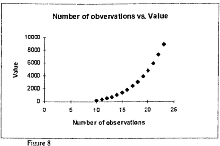
) !This value increases exponentially with increasing number o f observations, as in the figure'^ 8 in the appendix part. Therefore in large number o f observations, even with the fastest PC a data set with 75 observations may take days to finish the program. Therefore, the alternative solution which takes a shorter time is the random generations method.
3.2.1 Random Algoritm
The idea in the random algoritm is to generate a random index set and select the subsample according to that index. The trade-off between exacmess and randomness is that in random samples if you select a small number o f random generation you may miss the global solution. In the following sections we will try to show that the results o f random generation also produces satisfactory results.
In order to explain theorethically the possibility that also random generations produces good results we have to define e , which is the ratio o f bad data in the data set. We have the
following formula for the probability that the global solution is reached.
p _ I _ _ ^'^Variable number '•^Randcm Generaiiuns
We want this number
P
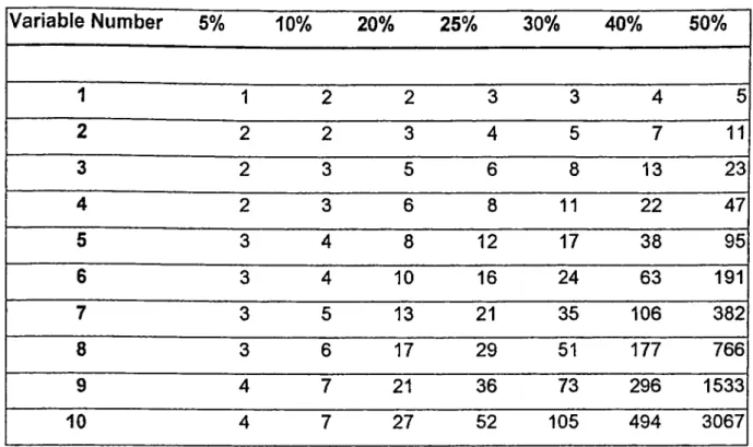
to be 95% or 99%, as large as possible. Table 2 below summarizes that how many numbers o f generations needed for the percent number o f contamined data to the dimension in hand if the observation number is very large compared to the variable number.Appendix page iii
Table 2.
Number of random generations needed in % contamined data
V a ria b le N um ber
5%
10%
20%
25%
30%
40%
50%
1
1
2
2
3
3
4
5
2
2
2
3
4
5
7
11
3
2
3
5
6
8
13
23
4
2
3
6
8
11
22
47
5
3
4
8
12
17
38
95
6
3
4
10
16
24
63
191
7
3
5
13
21
35
106
382
8
3
6
17
29
51
177
766
9
4
7
21
36
73
296
1533
10
4
7
27
52
105
494
3067
If we compate this table with the case that how many combinations is needed by exact solution we get Table 3 below.
Table 3. Number generation for exact solution for the given data number
2
3
4
5
10
20
40
V a riab le N um ber
1
2
3
4
5
10
20
40
2
1
3
6 10
45
190
780
3
1
4 10
120
1140
9880
4
1
5
210
4845
91390
5
1
252
15504
658008
6
210
38760
3838380
7
120
77520
18643560
8
45
125970
76904685
9
10
167960
273438886
10
1
184756
847660528
19We see that for a dataset o f size 20 and 4 variables, containing half o f bad observations the random generation requires 47 number o f generations while the exact solution requires 4845 number o f computations. The exact solition requires 10 times more computation. This however, does not imply that the random generations solution in computer is 10 times faster.
In most o f the computer programs there is no built in random number generaor that generates different numbers o f data for the given size. If you want to have a subsample with different indices than you have to spend some time on getting new indices for the dublicated ones. This decreases the ratio o f the exact time solution to the random from 10 to lower degrees.
The random generations in the program Robust work in the same principle as explained above. If we would explain it by a case assume that we have 15 observations and our subsample is o f the size 6. We first fill the matrix “indxit” with random index numbers,as below.
indxit = [\5
3 7 3 12 8]If the variable number is not negligible in comparison with the observation number, then the dublicated index numbers increases. The program, therefore, checks if the matrix has dublications in it. If the dublications are small in number, for example, 20% o f the total observations then it again tries six times to fill the dublicated ones with only one new generated index and checks if it is just before choosen.
If the duplications are in small number or if the observation number is large compared to the subgroup chosen then the above process is suitable. If however the subgroup element size is not small compared to the case number, generating an index and looking if it found before, and if it exists generate a new one may cause an infinite large trial and error loop. In this case it is more suitable to switch to a more guaranteed method o f filling the duplications. For this case we generate a new rest matrix “tester”, which is made up o f indices that do not exist in the first generated matrix “indxit”. For the matrix above we get the following matrix.
Tester = [\
2 4 5 6 9 10 11 13 14]i
In order not to lose the randomness property, from the rest matrix we randomly select one and add to the index matrix. For the example above we randomly generate a number o f 1 to the rest size, which is 10 in this case and select the index number there and add it to the index matrix.until the index matrix is filled. During this process the rest matrix shrinks in every trial by one. After the choice above the rest matrix becomes as follows.
rester = [\
2 4 5 6 9 10 13 14]3.3 Effectiveness
In this we will ask the question that if the random process is effective, because it has a shorter calculation time. The experiments performed are summarized in the tables in the appendix*^ and below. I have taken two extreme cases one is where observation number is very large compared to the variable number and one for which it is not negligible.
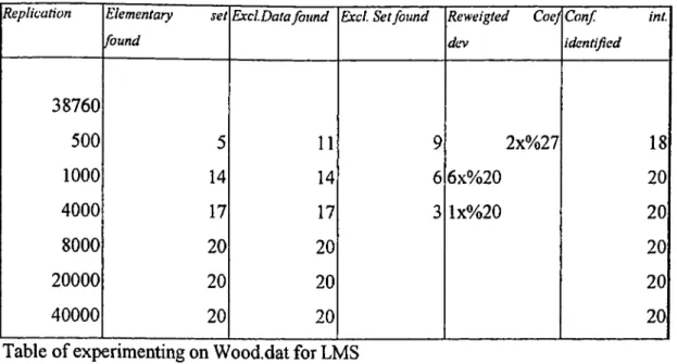
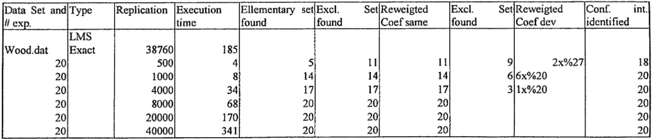
The first case is for Wood data set for which an observation number o f 20 against a variable number o f 4 exists. The results are summarized below. For the first table below we see that for replications below 8000 the estimated coefficients for the reweighted OLS differ but the significance level has only an error for replication below 1000.
To get the correct answer for the re weighted OLS we have to make at least 8000 replications because only after that we find the correct outliers. For the replication number below 8000 we get for the worst case a 20% deviation o f one o f the coefficients. For example, for 500 replications we have 9 results out o f 20, which have different coefficients than the exact solution. Two o f them have a deviation o f the coefficient from the true value o f 27%, more to that 18 results have identified the confidence interval correctly. Therefore, if you want to see the significance o f some coefficients you have to select a replication number larger than 500.
Appendix page 9,10
R eplica tio n E lem entary s e t fo u n d
E x c lD a ta fo u n d E xcl S et fo u n d R ew eig ted CoeJ d e v C o n f int. id en tified 38760 500 5 11
9
2x%27 18 1000 14 14 6 6x%20 20 4000 17 17 3 lx%20 20 8000 20 20 20 20000 20 20 20 40000 20 20 20Table o f experimenting on Wood.dat for LMS
The data set wood.dat is made up o f 20 observations and 4 variables and below we have the normalized data plot after LMS
Previously we have given numbers in Table 2, which was for the case that variable number was negligible with respect to observation number. We have to note that by looking at the figure we can see that there are no clear cut outliers, which makes difficult to find good subsamples.
As a result, if the number o f variables is relative to observation number not negligible, if the variables are spread or have high variance and if the number o f outliers is large we have to increase replication number up to degree o f 8000 replications, which is one fifth o f the replication number needed by the exact solution but takes two times less duration to be executed.
In the opposite extreme we have the data table o f the data set brainlog, which we often mentioned before. This case has three dinosaurs as clear outliers and 2 species that are ju st on the line. The next table summarizes that in all cases at least in one second you’ll get the correct result. This is so because all o f them correctly identify the outliers and get the expected result for reweighted OLS. This result is compatible with the suggestions o f table 2.
Replication Ellementary set
found
Excl.Data
found
Excl.
Set
found
Reweigted
Coef dev
Conf.
int.
identified
378 159
20 20 20 30 6 20 20 20 60 9 20 20 20 150 16 20 20 20 300 17 20 20 20The same fact is also true for that case also. As the MVE advices to take the elementary subset size as the variable number plus one(, which is one element more than the LMS or LTS). This in fact makes the execution time larger. It becomes also harder to find the correct elementary set. For the tables below we have the similar comments as above.
Type
Replication Execution time Ellementary
set
found
Leverage
found
pi Worst
possible
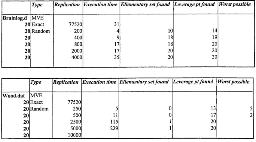
MVE Exact Random 77520 250 500 2500 5000 10000 1370 511
115 229 458 13 1720
20
20
As in the LMS part for the Brainlog data, we find in very few replications the target elementary set and leverage points. The execution time o f MVE is larger because it needs more calculation and has one more variable to account. However this is not the case for the Wood data, it happens for the few replications worst possible happens,i.e. it identifies no leverage point.
Type
Replicatio
n
Execution time Ellementary
set
found
Leverage
pt
found
Worst
possible
MVE Exact3216
31 Random 200 4 10 14 400 9 18 19 800 17 18 20 2000 35 20 20 4000 71 20 20Finally, the results obtained in random replications depend on the data set used. A data set with clear and small number o f outliers will give the result in replications few than the number o f fingers in a hand. In addition the variable number has to be negligible regarding the observation number. In contrast, if we have the opposite case it is preferable to use the exact solution.
4. Applications
In this section the idea that the outliera affect the results very much is investigated. Robust regression is applied on various data sets and the results are discussed. All data's are in the appendix part.
4.1 Urban Unincorporated Places
174.1.1 Extreme Case
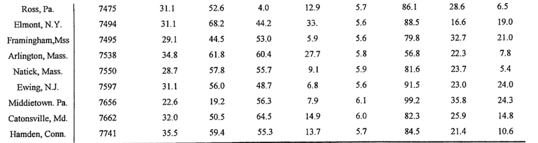
These data are taken form Country and City Data Book, 1962, Table 5, pages 468-475. They are examples for unincorporated places (with populations at least 25000), including the median family income for each. The last ten o f these are representatives for the 10 highest median income and the other ten for the lower ones. I have taken these as an example because o f the bias in selection and because the source I have taken used this also as an example.
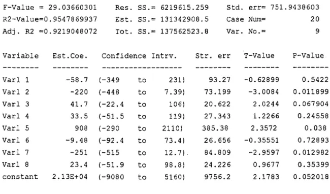
We get the following results;
F-Value = R2-Value=0 A d j . R2 =0 Variable 29.03660301 .9547869937 .9219048072 Est.Coe. Res. SS.= 6219615.259 Std. Est. SS.= 131342908.5 Case Tot. SS.= 137562523.8 Var.
Confidence Intrv. Str. err
err= 751. Num= No.= T-Value .9438603 20 9 P-Value Varl 1 -58.7 (-349 to 231) 93.27 -0.62899 0.5422 Varl 2 -220 (-448 to 7.39) 73.199 -3.0084 0.011899 Varl 3 41.7 (-22.4 to 106) 20.622 2.0244 0.067904 Varl 4 33.5 (-51.5 to 119) 27.343 1.2266 0.24558 Varl 5 908 (-290 to 2110) 385.38 2.3572 0.038 Varl 6 -9.48 (-92.4 to 73.4) 26.656 -0.35551 0.72893 Varl 7 -251 (-515 to 12.7). 84.809 -2.9597 0.012982 Varl 8 23.4 (-51.9 to 98.8) 24.226 0.9677 0.35399 constant 2.13E+04 (-9080 to 5160) 9756.2 2.1783 0.052018 17
Example taken from. Data Analysis and Regression, Frederick Mosteller & John W. Tukey
The author o f the given example claimed that Varl 4, which is % using public transportation, showing a relation in this multi-dimensional space. He comes to the strange conclusion that the more affluent are using more public transport by making the following plot.
As the evidence shows there seems to be a suprising relation between these variables. One has to ask the question that “are the richer rich because they are more stingy”. We see that the OLS could not identify any significance relation. After making the LMS and identifying the outliers we get the following results for OLS.
F-Value = 221.8849714 Re s . SS. = 481333. 6093 Std. err= 262. 2249877
R2-Value=0.9960720052 E s t , SS. = 122057936.1 Case Num= 16
Adj. R2 =0.9915828684 Tot. SS, = 122539269.7 Var. No.= 9
Variable Est.Coe. Confidence Intrv. Str. err T-Value P-Value
Varl 1 -67.7 (-211 to 75.7) 35.847 -1.8892 0.10079 Varl 2 -371 (-496 to -247) 31.158 -11.917 6.6631E—06 Varl 3 -4.61 (-57.1 to 47.8) 13.115 -0.35176 0.73537 Varl 4 37.5 (-2.93 to 77.9) 10.107 3.7104 0,007551 Varl 5 1760 ( 782 to 2730) 243.78 7.2065 0,00017645 Varl 6 -22,4 (-64.5 to 19,7) 10,533 -2.1265 0.071037 Varl 7 -394 (-529 to -259) 33.788 -11.656 7.7253E-06 Varl 8 22.5 (-12.1 to 57) 8.628 2,6023 0.035304
Constant 3.2E+04 ( 1.72E+04to4. 68E+04) 3692,2 8,6662 5.4508E-05
The results o f the reweighted OLS show that there is no relationship between % transportation and the income o f family. So people are not rich because the are stringy but because they have not moved to this city in recent years (Varl 8) and because they live in
suitable homes (Varl 5). In addition, they have changed their homes when they have changed their financial status (Varl2). OLS did not identify any o f these variables as significant and at the end there seem to be a wrong relationship, by intution. However, LMS picked up the most logical ones as significant out.
We can see from the figure that the outliers are from the linear trend (ellipses) and not from the possible outliers (dashed ellipse). So classical OLS and the author failed in this case.
4.1.2 More Data
If we add more intermediate data to the previous example in order to see what happens to the results we get the followings.
--- QL3 Results
---F-Value = 16,37391311 R e s . ss. = 17571075. 44 Std. err= 961..6618137
R2-Value=0 ,8733259904 E s t . ss. = 121139900 .0 Case Num= 28
Adj . R2 =0 ,8199895653 Tot. ss. = 138710975 .4 Var. No.= 9
Variable Est.Coe. Confidence Intrv. Str. err T-Value P-Value
Varl 2 155 (-74.6 to 384) 80 .07 1.9314 0.06849
Varl 3 -16.9 (-135 to 102) 41. 417 -0.40764 0.68809
Varl 4 15.7 (-29.5 to 60.9) 15.1 1 1 0.99446 0.3325
Varl 5 38.7 (-51.1 to 128) 31. 339 1.2336 0.23241
Varl 6 1.4E+03 ( 206 to2 .59E+03) 416 .11 3.3582 0.00330
Varl 7 32.5 (-41.7 to 107) 25. 908 1.2548 0.22478
Varl 8 -3.82 (-146 to 139) 49, 724 -0.076796 0.93959
Varl 9 37.1 (-28.8 to 103) 22. 996 1.6125 0.12334
Constant -8260 (-2,69E+04tol.04E+04) 6502 -1.27 0.2194
Reweighted OLS Results
Varl 2 Varl 3 Varl 4
196.1956855 R e s . SS. = 938049. 6419 Std. err= 279.5904210
.9924125810 Est. SS. = 122694195.0 Case Num= 21
.9873543017 Tot. SS. = 123632244.7 Var. No.= 9
Est.Coe. Confidence Intrv. Str. err T-Value P-Value
-48.6 (-142 to 44.7) 30 .483 -1.5953 0.13663
-377 (-467 to -287) 29 .329 -12.849 2.2497E-08
-3.3 (-20.5 to 13.8) 5. 6001 -0.59008 0.56608
Varl 5 40.5 ( 10.3 to 70.7)
Varl 6 1.61E+03 (1.13E+03to2.09E+03)
Varl 7 -18.4 (-46.3 to 9.45)
Varl 8 -396 (-497 to -295)
Varl 9 28.5 ( 5.81 to 51.3)
Constant 3.2E+04 (2.08E+04to4.32E+04)
9.8628 4.11 0.0014464 157.69 10.20 2.8814E-07 9.1051 -2.0242 0.065793 32.918 -12.035 4.6804E-08 7.4211 3.845 0.0023314 3655.9 8.750 1.4835E-06
Again, LMS has improved some variables but still leaving Var 4 insignificant. This example took 8 hours to get the exact solution. Additional data decreased precision o f the and standard error o f the OLS, but leaving the reweighted in almost same level o f precision.
4.2 Median Income and Population in US cities
18In this example we will use a large sample o f 146 cases. We have two cases, one with the ordinary data and one with the logarithm o f the data. The following figure is for the ordinary data with the results below.
0 200000 400000 600000 8 00000 Population 1000000 1200000 --- OLS Results F-Value = 15.01678080 Res. S S .=35835142273406 R2-Value=0.09443519563 Est. S S .=3737003309758 Adj. R2 =0.08314655116 Tot. SS.=39572145583164 Std. err= 498853.8410 Case Num= 146 Var. No.= 2 18
Example taken from. Data Analysis and Regression, Frederick Mosteller & John W. Tukey
Variable Est.Coe. Confidence Intrv. Str. err T-Value P-Value Population 93.8 Constant -2.66E+05 ( 30.6 to 157) (-5.53E+05to 2.1E+04) 24.217 109940 3.8751 -2.4201 0.00016133 0.01676
--- Reweighted OLS Results
F-Value = 4.332517245 Res. SS.= 15100337314 R2-Value=0.04036537441 Est. SS.= 635169629.3 Adj. R2 =0.03104853339 Tot. SS.= 15735506943 Std. err= 12108.06412 Case Num= 105 Var. No.= 2
Variable Est.Coe. Confidence Intrv.
Population 1.74 (-0.559 to 4.04) Constant 1.3E+04 ( 4190 to 2180) Str. err T-Value 0.83669 3204.4 P-Value 2.0815 0.03987 4.0564 9.709E-05
The case for the logarithmic plot follows with the results.
4 3.9 -C * 3.8 -0) i 3.7 J ♦ ♦ 1 3 . 6 - ♦ ♦ « . 1 3 · ^ ■ ■g 3.4 - . . * w 3.3 - ♦ 5 3.2 ^ ♦ 3.1 -3 --- 1--- 1---1 ---♦ ---♦ W ♦ ♦ ♦ ♦♦ ♦ ♦ 3.5 4.5 5 5.5 log(Population) 6.5
The results o f the logarithmic case are below.
--- QL3 Results F-Value = 80.04771624 Res. SS.= 33.82940551 R2-Value=0.3572797687 Est. SS.= 18.80532398 Adj. R2 =0.3528164338 Tot. SS.= 52.63472948 Std. err=0.4846920952 Case Nuin= 14 6 Var. No.= 2 Variable Est.Coe. log(pop) Constant 1.93 -2.41 Confidence Intrv. ( 1.36 (-4.42 to 2.49) to -0.387) Str. err 0.21526 0.77287 T-Value P-Value 8.9469 1.6515E-15 -3.112 0.0022412 29
Rev/eighted OLS Results F-Value = 131.6675077 Res. SS.= 20.56615765 R2-Value=0.4937515966 Est. SS.= 20.05047941 Adj. R2 =0.4900016084 Tot. SS.= 40.62463706 Std. err=0.3903100159 Case Num= 137 Var. No.= 2
Variable Est.Coe. Confidence Intrv.
log(pop) Constant 2.06 ( 1.59 to 2.53) -2.85 (-4.54 to -1.17) Str. err 0.17963 0.64277 T-Value P-Value 11.475 1.0729E-21 -4.4407 1.849E-05
I have selected these two cases for the following reason. The ordinary data with linear regression was a wrong choice. Actually, there is a tendency in the data showing that the larger the population size in the city the richer is the city. Possibly due to that fact the richer is the median family. The rule is not general but it is true for the most o f the cities.
Applying robust procedure for such a wrong linear model it throwed 41 data out o f 146, from the sample. This comes from the fact that the model is not linear. Looking back at the figure we see that there are a lot of rich medium income families living in small cities. This is a bit unusual, these cities may have an extra advantage than only depending on the population.
The choice of the log model is more logical, because as the population grows, growing wealth has to bedistributed. However the population grows faster. Wealth is attractive and therefore population size increases faster, because o f birth or emigration.
What does that mean? Does that mean that the LMS has failed, a more advanced technology produced wrong results. No, the LMS behaved correctly but the model was wrong. Therefore, LMS is able to detect in extreme cases wrong regression models. By using that fact, it is possible to write a program to find a better fit equation by using robust regression.
As a result, in regressions with missing variables or wrong model the robust procedures detects many points as outliers. This is another superiority o f the robust procedures. With this fact we can adjust our model but the classical OLS does not say anything.
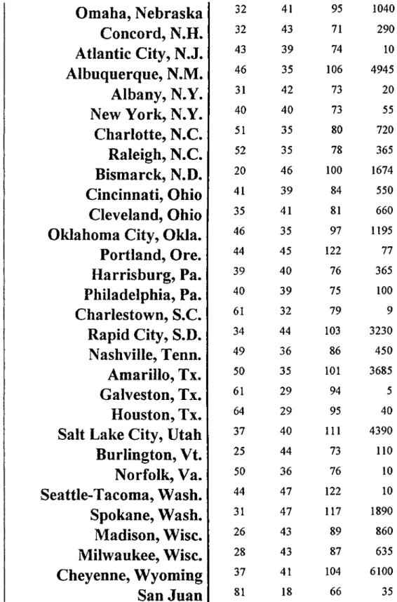
4.3 Latitude versus Temperature*^
This example is interesting i f we look at the figure below.
80 70 —
Maximum Januari» T e m p e r a t u r e vs. L a ti tu d e
♦ Jackso n ville 60 — ♦ ♦ ♦ ♦ ♦ ♦U^so —
0) k· 3*5
o5
40Q,
E
0 h 30^♦1
^ S eattle ♦ ♦ ♦ ♦ ♦ ♦ ♦ Junea 20 — 10 — H---l· 15 20 25 30 35 40 45 Latitude (degreees) 50 55 60 19Example taken from. Data Analysis and Regression, Frederick Mosteller & John W. Tukey
As you go south the temperature increases as expected. However, there are some outliers because o f their special position, to identify them we first look at the results.
F-Value = 86,97334953 Res. SS.= 2121.169555 Std, err= 6.100286957
R2-Value=0.8207096399 Est. SS.= 9709.748478 Case Num= 61
Adj. R2 =0.8112733051 Tot. SS.= 11830.91803 Var. No.= 4
Variable Est.Coe. Confidence Intrv, Str. err T-Value
Latitude -1.92 (-2.26 to -1.58) 0.1282 Longtitute 0.205 ( 0.079 to 0.332) 0.047442 Altitude -0.00176 (-0.00332to-0.000188) 0.000587 Constant 100 ( 82.8 to 117) 6.495 P-Value -14.958 2.1636E-21 4.3314 6.0722E-05 -2.986 0.0041604 15.408 5.5599E-22
All variables came out to be significant. The only outlier the OLS could identify was the Jacksonville. The results for reweighted OLS are.
F-Value = 665.1295723 Res. SS.= 182.0415429 Std. err= 2.011309927
R2-Value=0.9779453789 Est. SS.= 8072.080906 Case Num= 49
Adj. R2 =0.9764750709 Tot. SS.= 8254.122449 Var. No.= 4
Variable Est.Coe, Confidence Intrv. Str. err T-Value
Latitude -2.6 (-2,76 to -2.44) 0.05971 Longtitute -0.275 (-0,394 to -0.157) 0.043911 Altitude 0.00136 ( 0.000511to 0.00221) 0.0003157 Constant 163 ( 150 to 176) 4.7579 P-Value -43.554 1.9483E-38 -6.2733 1.2254E-07 4.3096 8.7848E-05 34.309 6.5764E-34
After throwing out 12 cases a better approximation is reached. This is a good example for the fact that the LMS is able to increase precision. The question remains to ask here is that if it is feasible to throw away 20% o f the data to get a better suited approximation.
We can say then that if the estimation we are going to make is for ordinary cities with no extraordinary position on the map then we can use the reweighted OLS, but if we are not sure that if the data we are using is corrupted or not, we can use both o f them for comparison. For e.xample, if I randomly select a data, which comes out to be Oklahoma City just to forecast. It has Latitude=35, Longtitude=97 and Altitude=1195. The OLS will give us a range o f 35.33 to 65.83 and for reweighted OLS 41.93 to 51.97, where the actual data was 46. In addition, while putting the data I forgot to put a possible outlier candidate, which is San Juan with Latitude=18,
Longtitude=66 and Altitude=35. Repeating the calculations we get for OLS the range 63.65 to 94.15 and for the reweighted OLS 93.07 to 103.34. The measured unit was 81 and there is a deviation in robust case.
We have to discuss that the results that why a robust regression produced an unexpected result. In fact it is not an unexpected result. Robust procedure has identified 20% o f the data as outlier, but most probably the data’s used are not corrupted or biased. Therefore, in one out o f five cases it is possible that robust procedure will fail in estimating the results. The results o f the OLS were also acceptable so we should not always use the robust estimation blindly just to increase the precision.
4.4 Education and Income
20The data for this case comes from 306 interviewed employees on city payroll. A random sample o f 32 people is selected out o f it and the following results are obtained.
OLS Results
F-Value = 39.87937474 Res. SS.= 242062725.4 Std. err= 2840 .555846
R2-Value= 0.5706887746 Est. SS.= 321777004.5 Case Num= 32
A d j . R2 =0.5563784004 Tot. SS.= 563839729.9 Var. No.= 2
Variable Est.Coe. Confidence Intrv. Str. err T-Value P-Value
Educatio 739 ( 388 tol.09E+03) 116. 94 6.315 5.8002E-07
Constant 4.99E+03 ( 514 LiMS to9.46E+03) 1490 Results .5 3.345 0.0022224 Variable Est.Coe. Educatio 956.5 Constant 966.0000000 R2=0.7128379090 Std err= 3332.371805
20Applied Regression An Introduction, Micheál S Lewis-Beck