KADIR HAS UNIVERSITY
GRADUATE SCHOOL OF SCIENCE AND ENGINEERING
OSCILLATIONS AND CHAOS IN GENE NETWORK
MODELS
B ÜŞR A A R IK AN M.S c. The sis 2017 S tudent’ s F ull Na me P h.D. (or M.S . or M.A .) The sis 20 11
OSCILLATIONS AND CHAOS IN GENE NETWORK MODELS
BÜŞRA ARIKAN
Submitted to the Graduate School of Science and Engineering In partial fulfillment of the requirements for the degree of
Master of Science In
COMPUTATIONAL BIOLOGY AND BIOINFORMATICS
OSCILLATIONS AND CHAOS IN GENE NETWORK MODELS
Abstract
BÜŞRA ARIKAN
Master of Science in Computational Biology and Bioinformatics Advisor : Assoc. Prof. CEM ÖZEN
July, 2017
Oscillations and chaos have always been interesting topics in the theory of dynamical systems. In systems biology, oscillations emerging from gene networks are known to be widespread as in circadian oscillations, various metabolic cycles and the cell cycle to name a few. According to the dynamical systems theory, chaotic behavior can also be produced in strongly-coupled gene regulatory networks (GRNs) with dimensions equal to or exceeding three. Although there is a large number of studies focusing on oscillators in systems biology, the number of studies on chaos is still rather limited. Therefore, much work is needed to understand the conditions for its occurence, its possible roles in nature and even novel biological functions which may allow for new biotechnological applications in future.
In this thesis, we are interested in the chaotic dynamics emerging from a couple of small gene networks capable of exhibiting chaotic dynamics. Using different approaches, we investigated the parameter space of these network models for configurations that yield chaotic solutions. Our findings indicate that although such solutions exist, they are rare and isolated to the boundary separating the regions of the fixed-point and oscillatory dynamics in the multi-dimensional parameter space. This finding is compatible with the result of a recent study in the literature in which the same genetic circuits were studied but in a more restricted parameter space.
We also investigated the topic of chaos control in the systems we have considered. Chaos control is a term for methodologies that are used to stabilize chaotic dynamics and is rather young sub-discipline of the control theory. Using one of the most well-known control approaches, the Pyragas method, we have demonstrated that chaotic behavior can be stabilized by an application of a small perturbation in the form of a feedback to the original system. Beyond the scope of this thesis, we aim to extend the control approach to develop a biologically feasible control method that may be used in the future biotechnological applications.
Keywords: Dynamical Systems, Gene Regulatory Networks, Systems Biology,
GEN AĞ MODELLERİNDE OSİLASYON VE KAOS
Özet
BÜŞRA ARIKAN
Hesaplamalı Biyoloji ve Biyoinformatik, Yüksek Lisans Danışman: Doç. Dr. CEM ÖZEN
Temmuz, 2017
Osilasyonlar ve kaos dinamik sistemler teorisinde her zaman ilgi çeken konular olmuştur. Sistem biyolojisinde, gen ağlarında ortaya çıkan osilasyonlar, sirkadiyen osilasyonlar, çeşitli metabolik döngüler ve hücre döngüsü gibi bir çok alanda yaygın olarak bilinirler. Dinamik sistemler teorisine göre, kaotik davranış, boyutları üç ve üçün üzerinde olan güçlü-bağlı gen düzenleyici ağlarda(GRNs) da gözlemlenebilir. Ancak, sistem biyolojisinde osilatörler üzerine yapılmış bir çok çalışma bulunurken, kaos üzerine yapılan çalışma sayısı hala oldukça sınırlıdır. Bu nedenle, kaosun oluşum koşullarını, doğadaki muhtemel rollerini ve hatta gelecekte yeni biyoteknolojik uygulamalara yön verecek özgün biyolojik fonksiyonlarını anlamak için daha çok çalışmaya ihtiyaç vardır.
Bu tezde, kaos oluşturabilen birkaç küçük gen ağında ortaya çıkan kaotik dinamikleri ele aldık. Farklı yaklaşımlar kullanarak, bu ağ modellerinin kaotik çözümler üreten konfigürasyonları için parametre uzayını araştırdık. Bulgularımız, bu çözümlerin varolmasına rağmen, nadir olduklarını ve çok boyutlu parametre uzayında sabit nokta ve osilatif dinamikleri ayıran sınırlarda izole olduklarını gösterdi. Bu bulgu, aynı genetik devrelerin daha kısıtlı bir parametre uzayında çalışıldığı literatürde yapılan yeni bir çalışmanın sonucuyla uyumludur.
Ayrıca, incelediğimiz sistemlerde kaos kontrol konusunu araştırdık. Kaos kontrol, kaotik dinamiklerin kararlı kılınmasında kullanılan metodolojiler için bir terimdir ve kontrol teorisinin oldukça genç bir alt disiplinidir. En iyi bilinen kontrol yaklaşımlarından biri olan Pyragas yöntemini kullanarak, kaotik davranışın, orijinal sisteme geribildirim şeklinde küçük bir pertürbasyon uygulayarak kararlı kılınabileceğini gösterdik. Bu tezin ötesinde, gelecekteki biyoteknolojik uygulamalarda kullanılabilecek biyolojik olarak uygulanabilir bir kontrol yöntemi geliştirmek için kontrol yaklaşımını genişletmeyi amaçlıyoruz.
Anahtar Kelimeler: Dinamik Sistemler, Gen Düzenleyici Ağlar, Sistem Biyolojisi,
Acknowledgements
More than anything, I would like to express my sincere to my advisor Assoc. Prof. Cem Özen for being such an excellent educator. I would like to thank him for his contributions to both my personality and my research career. I could not complete this thesis without his patience and support.
Besides my advisor, I would like to thank my committee members: Assoc. Prof. Kutsal Bozkurt and Asst. Prof. Hatice Bahar Şahin for their confidence and comments. I also would like to thank the other teachers at Kadir Has University Department of Bioinformatics and Genetics for their contributions to my education.
Finally, I owe more than thanks to my parents Ahmet and Nermin Arıkan, and my sister Kübra Arıkan Uğurlu for their priceless love and support. They did everything to make sure I received the best education possible and they always believe in me. Without them I would not be the person I am now.
Table of Contents
Abstract………..i Özet………..iii Acknowledgements………...v Table of Contents………vii List of Tables……….………….viii List of Figures……….………….ix List of Abbreviations………..…………...x 1 INTRODUCTION………..…………...11.1 WHAT IS SYSTEM BIOLOGY ?………..………….3
1.2 GENE REGULATION………..…………..4
1.3 MATHEMATICAL MODELLING AND GENE NETWORK DYNAMICS……….………..…………...7
1.3.1 Classification of Dynamic Behavior………..………...10
1.4 OSCILLATION AND CHAOS IN GENE NETWORKS……….13
2 METHODS………...16
2.1 CHAOTIC MODELS………16
2.2 CLASSIFICATION OF DYNAMIC FEATURES………17
2.2.1 Calculation of Lyapunov Exponents………...17
2.2.2 Bifurcations……….21
2.2.3 Lyapunov Spectrum of Dynamical Systems………...23
2.3 PARAMETER ESTIMATION………..26
2.4 CHAOS CONTROL………..34
3 RESULTS AND DISCUSSION………...38
3.1 GRN MODEL SELECTION……….38
3.2 SEARCH FOR CHAOTIC DYNAMICS IN THE PARAMETER SPACE……….40
3.3 BIFURCATION PLOTS AND THE LYAPUNOV SPECTRA……….45
3.4 CHAOS CONTROL………..48
List of Tables
Table 1.1: Mathematical expression of transcriptional regulation………9 Table 1.2 : Some of the important biological oscillatory process………...14 Table 2.1 : Classification dynamic features by calculation maximum Lyapunov
expo-nent………..18
List of Figures
Figure 1.1: Central dogma of biology………..5
Figure 1.2: Transcriptional regulation of gene expression………...6
Figure 1.3: Dynamic behaviors of systems at the level of a system component………11
Figure 1.4: Decomposition of two trajectories over time in a chaotic system………...11
Figure 1.5: Random, regular and chaotic mechanisms………..12
Figure 2.1: Bifurcation diagram of Rössler system………22
Figure 2.2: 3D phase space images of Rössler system………...23
Figure 2.3: The Lyapunov spectrum of the Rössler system………...24
Figure 2.4: The Lyapunov spectrum of the Rössler system………...24
Figure 2.5: Determination of system dynamics by Lyapunov exponents………..25
Figure 2.6: Parameter estimation by using UKF………30
Figure 2.7: Sensitive parameter estimation with the UKF filter……...……….32
Figure 2.8: A constrained-parameter search using the UKF method……….34
Figure 2.9: Feedback-based chaos control scheme in Pyragas method……….35
Figure 2.10: Using the Pyragas method on the Rössler model………..36
Figure 2.11: Using the Pyragas method on the Rössler model 3D……….37
Figure 3.1: GRN Motif………...39
Figure 3.2: Scanning the parameter space on selected 2-D projections………41
Figure 3.3: Constant K plane………..42
Figure 3.4: Constant K2 plane………43
Figure 3.5: Constant K1 plane………44
Figure 3.6: Bifurcations and Lyapunov spectra of the GRN model………...45
Figure 3.7: Samples of circuit motifs taken from (Suzuki 2016)………...47
Figure 3.8: Power spectrum of GRN model………...48
List of Abbreviations
DNA deoxyribonucleic acid
RNA ribonucleic acid
mRNA messenger RNA
TF transcription factor
GRN gene regulatory network
ODE ordinary differential equations
FL feedback loops
NFL negative feedback loop
PFL positive feedback loop
ECG electrocardiogram
EGG electroencephalogram
1 INTRODUCTION
Most cellular functions are carried out by proteins. Protein concentrations within cells are time-dependent functions. Mathematically speaking, the rate of a protein’s concentration change depends on the competing production and degradation rates. While the degradation rate can be simply due to the cell growth or the additional activity of active agents (such as proteases), the production rate may depend on a number of factors related to the machinery of transcription and translation. It can be said that not single genes but this machinery is mainly responsible for the complex world of biology. In particular, if single genes are likened to an electronic circuit’s elements, many biochemical processes associated with these genes and their products can be likened to the wirings of the electronic circuit. Differences between two species sharing a large number of genes, such as humans and chimpanzees or even humans and yeast is largely attributable to the difference in the wirings of these species’ genomes rather than the small number of different genes. Hence, one arrives at the concept of gene circuits whose overall function depends on a system level understanding, and cannot be reduced to the sum of the behavior of its constituent genes.
Theoretical system biology is the branch of biological sciences focused on understanding the working principles of such systems through mathematical modeling and computational methods. One of the most common mathematical modeling approaches is the formalism of dynamical systems which describes the system as a set of differential equations, each of which representing the rate of concentration change of a system variable. The resulting system of equations are in general coupled, first order ordinary differential equations (ODEs). Using standard computational methods one can integrate these equations starting from a given set of initial values. This way, one obtains trajectories in the state space of system variables, uniquely determined from the system equations and initial conditions.
In this thesis, we investigate the emergence of chaotic dynamics and its control in some GRNs which are expressed as dynamical systems. In general, dynamical systems are classified according to the type of behavior its trajectories settle in the limit of long time. Accordingly, the systems could settle to a fixed-point, an oscillatory trajectory or a chaotic trajectory. Among these behaviors, oscillations and chaos are usually the more interesting from a mathematical as well as biological point of view. To date, a large number of oscillating networks have been identified in systems biology with the circadian rhythms, mitosis, cyclic AMP production in signaling being just a few well-known examples (Novak 2008). Mathematical models of these systems have been studied since the 1960s (Goodwin 1965).
Dynamical systems of dimension equal to or exceeding three can exhibit chaotic dynamics if the system is strongly coupled and sufficiently nonlinear. Chaotic systems exhibit aperiodic behavior that is also characterized by an extreme sensitivity to initial conditions. Variability in such systems sometimes can be confused with randomness, although the systems are perfectly deterministic. Unlike the case for oscillators, the relevance of chaos in systems biology still remains a largely open question. The first problem is practical: observing chaos in gene expression data is extremely challenging due to noisy cellular environment. So far, it has not been possible to obtain an experimental evidence for chaos in gene networks to our knowledge. Another question is rather functional: assuming that chaotic gene networks exist, how can a random-like dynamical behavior be useful in a biological system. Could there be any useful function for chaotic dynamics that might have been discovered by natural evolution? Or perhaps, could it be a manifestation of a diseased state such as cancer? Yet another possibility is a synthetic one: can one identify an altogether novel function for chaos which may create opportunities for future biotechnological applications as in synthetic biology. While these questions remain mostly speculative at the moment, there are a few studies in the literature addressing some aspects of these questions. As an example, recently Zhang et.al (Zhang 2012) investigated the abundance of chaotic solutions in randomly
generated small gene networks to identify whether there are chaotic networks that are more likely to occur in biological systems than pure chance would dictate.
In this thesis, we have investigated some of the GRNs identified in Zhang 2012 as capable of exhibiting chaotic dynamics. To differ from Zhang 2012 study, we expanded the parameter set of the mathematical models to provide greater dynamical behavior range to these systems. Subsequently, we have searched the parameter space of the model for discovering sets of parameters that yield chaotic solutions. Our results indicate that although such solutions can be found, they are isolated and confined to the boundary between domains of fixed point and oscillatory dynamics. We have also investigated the applicability of a chaos control method in the networks we examined. Chaos control refers to a purposeful manipulation of a system exhibiting chaotic dynamics with the aim of stabilizing the system. Typically such a control is performed using a feedback control mechanism to stabilize a particular regular orbit embedded within the chaotic set of solutions, known as the chaotic attractor. The motivation for controlling chaos in gene networks stems from a growing number of engineering applications, such as secure electronic communications and fast decision making systems in robotics (Feki 2003; Steingrube 2010).
1.1 WHAT IS SYSTEM BIOLOGY ?
Biological systems are composed of thousands of elements and exhibit complex behav-ior. The organization and function of these elements in the cell is a result of millions of years of evolution. The hierarchy of complexity continues to grow from one cell to the organism with layers of intercellular and intracellular interactions. Every living organ-ism keeps the information necessary for its survival in the genetic metarial, DNA. Most cellular functions such as cell growth, cell division, response to external stimuli, are managed by the action of proteins, which are expressed from the genes.
Through the advances in molecular biology techniques not only the genes and proteins but also their functions have been rapidly deciphered in recent years. However, it is clear that to understand the complexity of biological systems requires more than under-standing their components, so that a system-level underunder-standing is essential in this en-deavor. Almost all biological function emerges at the system level. Processes such as growth, proliferation, differentiation, response to a stimulus occur as a result of interac-tions among many cellular components. System biology tackles the problem of under-standing of the emergent properties of biological systems by way of mathematical mod-eling and computational methods (Kitano 2002).
1.2 GENE REGULATION
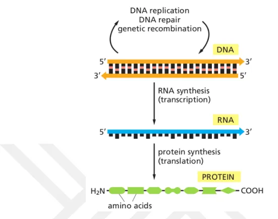
Cells are the basic units of life. By the differentiation and association of the cells, more advanced organisms are formed. For this reason we need to start from the cells to under-stand the living things. Decisions such as the growth, differentiation, death or prolifera-tion of a cell are regulated by funcprolifera-tional proteins. Conversion of hidden code in genetic material into active proteins constitutes the gene expression. Gene expression occurs in two steps, transcription and translation. Transcription is the RNA synthesis step from DNA in the nucleus. Translation is the synthesis of protein from messenger RNA in the ribosomes which found in cytosol. The addition of DNA replication, which is the process of making a new DNA from existing DNA, defines the central dogma of the bi-ology (Figure 1.1).
Figure 1.1: Central dogma of biology. DNA replication, transcription and translation (Alberts 2014).
Although all the cells of an organism have the same genome, they have to make differ-ent gene expressions according to the functions of the cells in differdiffer-ent regions and tasks. Hence gene regulation is the basis of function of biological mechanisms.
The conversion of a gene to active protein is controlled in many steps within the cell. First, transcription of a gene is regulated by the recognition and binding of specific re-gions (promoter) of the protein, which are called transcription regulators and constitute the largest class of proteins in cells (Alberts 2014). While transcriptional activator pro-teins enhance or induce gene transcription by the RNA polymerase, transcriptional re-pressor proteins prevent or suppress gene expression. Although this system in prokary-otes generally works in a wide on-off form, the gene control region of eukaryprokary-otes con-tains the sequence to which multiple transcription regulators can bind at the same time. Many transcription regulators work together to determine which gene, when, and to what extent transcription will occur.
In addition, a gene product is seen in many biological mechanisms in which it functions as its own transcription regulator. The control mechanisms by which a gene product in-hibits its own transcription are called negative feedback loop (NFL). Conversely, the mechanism by which a gene product activates its own transcription is called positive feedback loop (PFL).
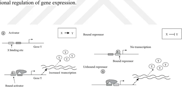
Although transcriptional regulation is the most important control step in the translation of a protein, subsequent control steps are also effective such as transport of molecules between cell compartments, degradation reactions, complex formation, etc. Mathemati-cal models are shaped according to the subjects to be investigated. These intermediate steps can be added to the model. In this study we will examine models based on the im-portance of transcriptional regulation. Figure 1.2 shows a general graph for transcrip-tional regulation of gene expression.
Figure 1.2 : Transcriptional regulation of gene expression. Transcription begins by binding the RNA
polymerase to the promoter region of the Y gene. X is trancription factor (TF) of gene Y. Transcription is increased by binding the activator X to the promoter region(left). Conversely, attachment of repressor X
1.3 MATHEMATICAL MODELLING AND GENE NETWORK DYNAMICS
A model briefly refers to the simplified representation of a real system. Making mathe-matical models that can explain observed biological phenomena or experimental results informs us both the ability to ask more questions about the system we are searching for and the freedom to answer more questions by leaving the challenge and expense of ex-perimental work aside.
Mathematical modeling of a biological system are usually classified into deterministic and stochastic type of models. The deterministic models treat system variables as con-tinuously changing quantities whose future values can be uniquely calculated using a precise set of mathematical expressions and initial conditions. Stochastic models on the other hand take various sources of noise, external and internal, into account. Although they are in general more realistic than the deterministic models, their solutions are often more difficult and their results are comparatively not easy to interpret. For such reasons, in this thesis, we have used a on a deterministic approach.
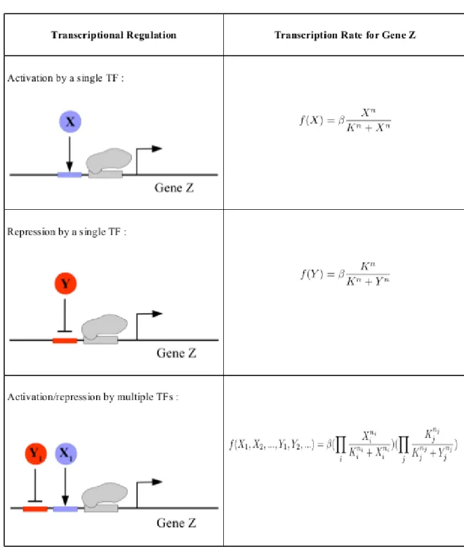
A cell is a dynamic system consisting of thousands of interactive elements. In order to understand how the dynamic system develops over time, we can construct ordinary dif-ferential equations (ODE) that indicate the rate of change in the state variables of the system. Accordingly the change of a component over time depends on the rate of gain and loss. When we think of gene networks, processes such as synthesis, degradation, complex formation, transport between cell parts, and chemical modifications determine the gain-loss rate of a component over time. However, the most important regulation mechanism gene networks is of the transcriptional kind. For this reason, in this thesis only transciptional regulation through the action of activator and repressor proteins have been considered to keep the problem as simple as possible.
In the description of transcriptional regulation, we have used the so called Hill func-tions, which can be derived from the law of mass action or more formally using the thermodynamic equilibrium. Suppose that the transcription of a gene Z is controlled by the transcription factor X. Transcription rate of gene Z is a function dependent on the concentration of X, .
If gene Z transcription is controlled by more than one transcription factor, transcription rate can be described by a multi-dimensional Hill equation, , and formaliza-tion depends on the specifics of the promoter of the gene. If all TFs are needed to start transcription and they act independently to each other, it is similar to AND gate.
In this thesis, we have made the choice of employing AND logic to describe the regula-tion of a gene by multiple transcripregula-tion factors. The detailed diagrams of these mecha-nisms and the corresponding equations for the transcription rates are shown in Table 1.1.
Table 1.1: Mathematical expression of transcriptional regulation. is activation / repression coefficent , is the maximum expression level of the gene and is Hill coefficient, larger creates more step-like motion in the S-shaped Hill function which indicates cooperative effects. typically takes values
For a more detailed discussion of the gene regulation, one can refer to many publica-tions. For example, see Alon 2007, Ingalls 2013, Klipp 2016.
1.3.1 Classification of Dynamic Behavior
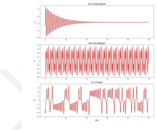
Using biochemical reaction kinetics, biological systems can be written a set of ODE, which describes a dynamical system. We assume that being physical systems, these systems are attractive dynamical systems, that is, their solutions are always confined to a finite region in the space of their stata variables. In the theory of dynamical systems, attractive dynamic systems are classified according to the limit sets of solution, that is, the set of state point(s) the system will settle to, after a sufficiently long period of time. These dynamic behaviors are stable fixed point, an oscillatory solution or a chaotic at-tractor (Figure 1.3).
Stable Fixed Point : System collapses to a single point in the phase space. It is the
point where f(X) is fixed for all time t (where t is sufficently long).
Oscillation : A periodic trajectory in the phase space, which is usually a limit cycle, a
periodic trajectory on which all nearby trajectories converge in sufficiently long periods of time.
Chaos : Trajectories are attracted to a limit set of points in the phase space, which is
called a strange attractor. Trajectories on the strange attractor are aperiodic, and in ap-pearance they look like random. Another feature of chaotic dynamics is the extreme sensitivity on initial conditions, so that two initially nearby trajectories will diverge from each other eventually (Figure 1.4).
Figure 1.3 : Dynamic behaviors of systems at the level of a system component. The x-axises indicate
time(s) and the y-axises indicate concentration of one of the components in the system for each plot. a) Fixed-point dynamics, b) oscillatory behavior, c) chaotic dynamics.
Figure 1.4 : Decomposition of two trajectories over time in a chaotic system, initiated from two points
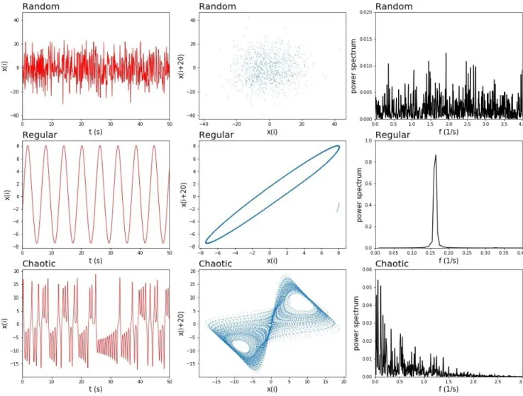
A distinguishing feature of a chaotic time-series from a random time-series is that when the element is plotted versus the element, a chaotic time-series produces a pattern that shows non-zero correlations that are not present in the case of the random time-series (Liebovitch 1998). Another difference between chaotic and random pro-cesses can often be observed in the structural differences between their respective power spectra. Despite the presence of an infinite number of peaks in both, there are also correlations governing the distribution of peaks in case of chaos, that are again missing in the random case (Figure 1.5).
Figure 1.5: Features of random, regular and chaotic mechanisms. Each column contains a plot for
ran-dom, regular and chaotic behaviors. The columns show the time series data sets, the phase space sets and the power spectra of the three mechanisms, respectively.
1.4 OSCILLATION AND CHAOS IN GENE NETWORKS
In vivo, most of the genetic and metabolic intracellular and intercellular regulation is homeostatic. This is achieved by adaptation of important parameters according to changing environmental conditions such as reaction speed. Lost of the balance leads to many injuries and illnesses for the living. Recognizing biological regulatory systems, describing the system where the behavior is necessary, and classifying the its character will guide us when we are able to control these systems, avoiding diseases, treating, or even creating synthetic mechanisms.
The motif idea has recently attracted considerable interest in gene regulatory network (GRN) studies because a network motif is thought to be a key feature of its function. GRNs have common character and network structure. For example, PFLs and NFLs are found in many biochemical networks and in important gene regulatory systems. The studies also support the idea, for example, that oscillation-based systems often have a negative feedback control, or that swicth-like movement usually occurs with a positive feedback control.
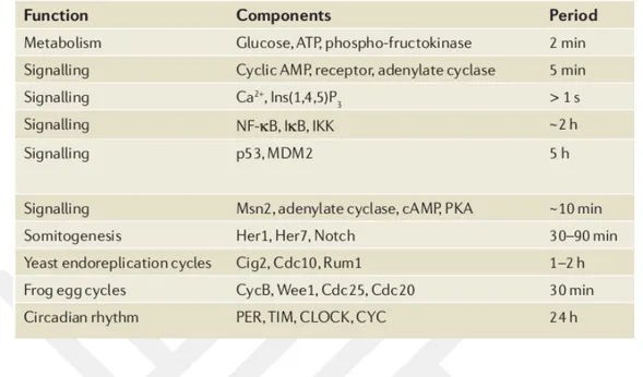
Especially oscillations are the most effective elements in anticipating biochemical many processes and providing homeostasis in minute, daily, even monthly periods. Such as glycolysis, mitosis, circadian rhythms, which fulfill important functions for the cell, are structures based on feedback loops (FL). Table 1.2 gives examples of oscillators in im-portant functions in the cell.
Table 1.2 : Some of the important biological oscillatory process (Novak 2008).
Since gene regulatory networks are known to contain more than one and associated os-cillators, complex nonlinear behaviors such as chaos can also be expected in those with more than three component. While there is such a high probability, the rare occurrence of chaos in GRNs is still an unanswered question.
In some of the studies in which the chaos theme was examined, chaos was found both as experimental and simulated in chemical reactions (Furusawa 2009). Are there chaos in gene regulatory systems? If so, what is its role? There are a few studies trying to an-swer these questions. Zhang et al. showed the presence of chaotic motifs in GRNs in their research published in 2012, which investigates the relation of chaotic dynamics to the structure of the system.
One of the findings of Zhang 2012 is that chaotic dynamics usually emerges with the competition between two or more oscillatory components. They also suggest that motifs that produce chaos also require very particular choice of system parameters and they attribute the rareness of chaos to this reason. Beyond the scope of Zhang et al., the fol-lowing questions are also important for future: Is there a mechanism to protect GRNs
from chaos, or do GRNs use chaos in a controlled way? To answer these questions, it is necessary to conduct further research on this subject.
Chaotic models have been shown to be more robust to cellular noise and mutation than other models. Robustness is a term used to define how much a system can protect its function in varying conditions. Systems that are overly sensitive to structural or envi-ronmental changes are not suitable for biological or other dynamic systems. Robustness is an important feature for biological systems, considering how complex the cellular events are. Returning to the topic of chaos, if GRNs contain and benefit from such dy-namics, these networks must also contain robust attractors with respect to variations in system parameters.
Lastly, if genetic systems display chaotic dynamics, is it used to a useful end in a process such as the differentiation, adaptation or provision of equilibrium? Or is it, as suggested by some scientists, associated with the onset of cancer? The answers to these questions are still largely unknown and further research is needed to clarify it.
2 METHODS
2.1 CHAOTIC MODELS
The approaches and algorithms we will discuss in the method section are designed to address different problems and complexities. The work we are trying to do here is a multidisciplinary approach that brings together the laws of physics, mathematics and bi-ology. Before attempting on a direct application to the biological problem at hand, for reasons of testing the algorithms and their accuracy, we have performed a number of studies on toy models which have been extensively studied in the literature. The result of these studies have been reported in this section.
The first of these toy models is the Lorenz model, which was first proposed by Edward N. Lorenz, a meteorologist, for his work on very-long-range weather prediction in 1963. This system, which consists of 3 coupled differential equations and has 3 variable pa-rameters, has been used as an example of deterministic chaos in many studies including the methods to be shown below(Wolf 1985; Rosenstein 1993; Silk 2011).
The other toy model we use is known as the Rössler model which was proposed by the mathematician Otto Rössler for studies on chaos in 1976. This system, also contains 3 variables and 3 parameters as in the Lorenz system and is described by the following set of equations:
2.2 CLASSIFICATION OF DYNAMIC FEATURES
2.2.1 Calculation of Lyapunov Exponents
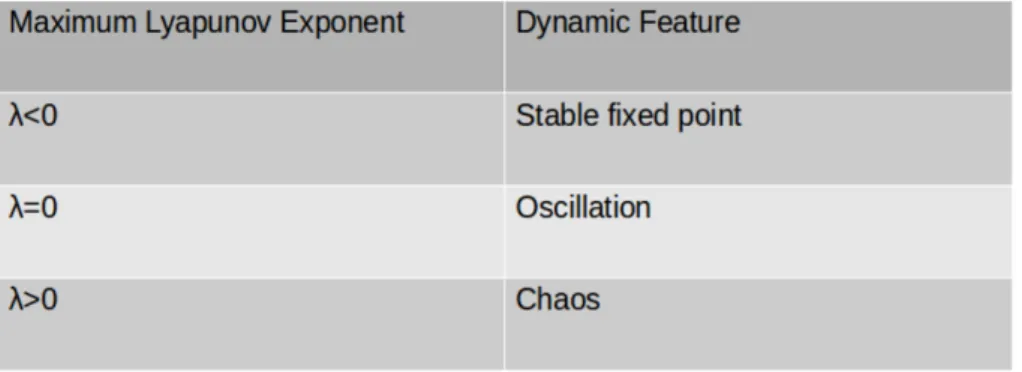
In the theory of dynamical systems, Lyapunov exponents are measures of average expo-nential rate of convergence (or divergence) between two trajectories which started from two initial points that are very close to each other. In an n-dimensional system, there are n Lyapunov exponents . The largest of these is the measure of the least stable direc-tion and by itself sufficient for characterizing the system dynamics. Table 2.1 summa-rizes the dynamic behavior of the system according to the value of the maximum Lya-punov exponent.
Table 2.1 : Classification dynamic features by calculation maximum Lyapunov exponent
There are different methods for calculating Lyapunov exponents. One of the most well-known of these is the Rosenstein algorithm proposed by Rosenstein et al. in 1993 for finding the maximum Lyapunov exponent from time series (Kantz 2003).
As an advantage to many other methods, this approachdoes not require one to know the systems dynamical equations. Thus, it was particularly useful for studies in which only data in the form of times series is available, as in electrocardiogram(ECG) and electroencephalogram(EGG) data. However, as a downside, the determination of the (maximal) Lyapunov exponent requires a curve-fitting process which requires human involvement. Therefore, the applicability of this method turned out to be rather restric-tive for a large number of such computations that we intended to do in this thesis.
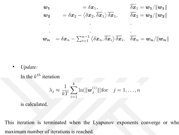
As an alternative to the Rosenstein method, there are also approaches in the literature in which the Lyapunov exponents can be determined using a recursive computation. The Bennettin algorithm is one such method, and can compute not only the maximum but all of the Lyapunov exponents. Contrary to the Rosenstein method, the Benettin method requires the knowledge of the system equations and also do not follow a curve-fitting procedure (Parker 1989).
The Benettin algorithm is based on the principle that the variational equation
is integrated simultaneously with the dynamical system itself, , for a short pe-riod of time . Here we use the initial conditions of and the orthonormal vectors. Here, represents the Jacobian matrix. The steps of the algorithm are as follows:
• Initial value assignment:
and orthonormal are selected. Then,
the following steps are performed iteratively. • İntegration:
In the instance, the system
is integrated during time with conditions and to obtain and . The new vector is usually not orthonormal.
• Orthonormalization:
In the iteration, the orthonormal is obtained with the Gram-Schmidt orthonormalization from the nonorthogonal vector :
• Update:
In the iteration
is calculated.
This iteration is terminated when the Lyapunov exponents converge or when the maximum number of iterations is reached.
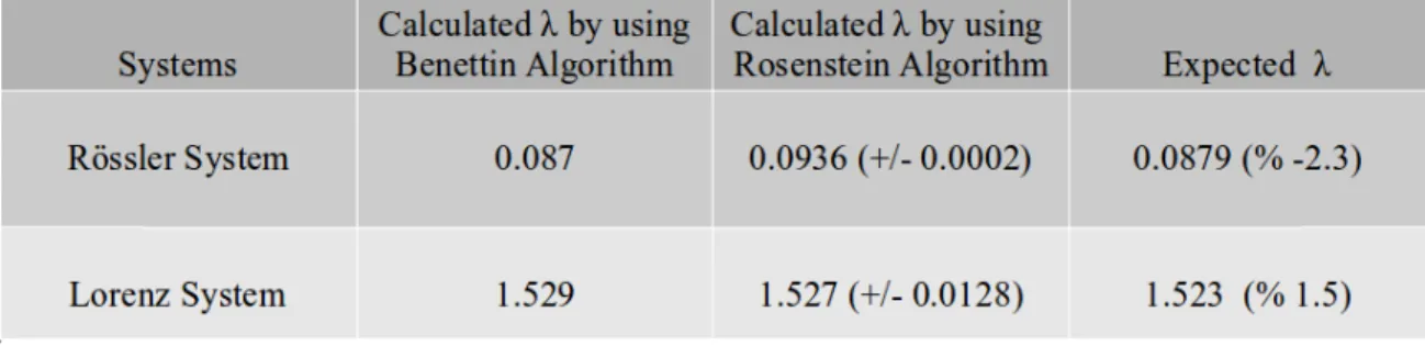
Table 2.2 shows that the maximum Lyapunov exponents ( ) calculation is made using both the Benettin and Rosenstein algorithms, and the expected values. Two algorithms give very comparable results. We have tried these calculations on the Lorenz and Rössler systems, which have been used in many Lyapunov calculation studies. The cal-culations we have made with previously published and commonly used parameter val-ues showing chaotic dynamics show that both methods can be successfully used. For the experiments we have made much more detailed, we assume that the following table gives a summary view. The Rosenstein algorithm has been used as a control in order to increase the reliability of the work we have done for the special points we have found in our further studies.
Table 2.2 : Comparison of results of two Lyapunov calculation methods with reference values of
maxi-mum Lyopunov exponents for Rössler and Lorenz systems.
2.2.2 Bifurcations
We know that the qualitative properties of the dynamics depends on the parameter val-ues as well as the initial conditions. Bifurcation analysis is one of the most commonly used approaches to study the change in the qualitative behavior of the system. In bifur-cation diagrams, asymptotically visited values of a chosen state variable is plotted against changing values of a system parameter, which is called the bifurcation parame-ter. All other parameters of the system is kept constant. In the following, we use the ap-proach that when the system is in an oscillating dynamics, we pick the peak value of the oscillating state variable’s values to be plotted against the bifurcation parameter. De-pending on the topology of the limit cycle, in oscillatory dynamics one can find one, two, three, .. peaks, corresponding to period-1, period-2, period-3 oscillations.
When the dynamics become chaotic, the asymptotic time series become aperiodic, therefore the number of peaks become infinite and corresponding to a given bifurcation parameter value, one obtains a continuum of peak values. Lastly, when the dynamics is of fixed point type, there would be no local variability in a state variable’s values, hence no peak value can be assigned, as such we, by convention, omit fixed points in these plots.
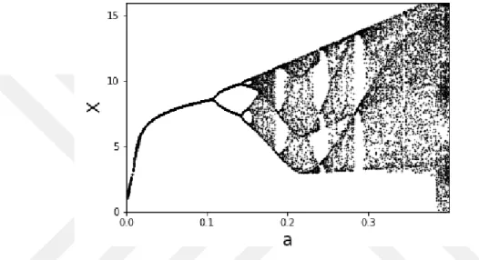
In Figure 2.1 we show the bifurcation diagram of the Rössler system with respect to the parameter 'a' of the Rössler system. While the 'a' parameter indicates that the system ex-hibits an oscillatory behavior at small values (a < 0.1), it is later seen that the period doubling into complex dynamics and chaotic transformation has occurred.
Figure 2.1: Bifurcation diagram of Rössler system’s first component X when parameter ‘a’ varied in the
range [0-0.4] and other parameters are constant (b=0.20, c=5.7): x-axis indicates parameter values and y-axis indicates X peak values.
In Figure 2.2, we plot the asymptotic trajectories of the Rössler system in its 3-D phase space. Each subplot corresponds to a particular choice of the bifurcation parameter that were used in Figure 2.1. These figures show the onset of chaos while the system goes through a series of bifurcations, involving what is called period-doubling bifurcations, which is a well-known route to chaos in dynamical systems theory.
Figure 2.2 : 3D phase space images of Rössler system with choosen ‘a’ values at bifurcation diagram
Figure 2.1. Other two parameters are fixed at same values in Figure 2.1: a) a=0.1, a periodic limit-cycle, b) a=0.12, a period two cycle, c) a=0.15, a period four cycle, d) a=0.2, a chaotic attractor.
2.2.3 Lyapunov Spectrum of Dynamical Systems
Another way of showing the qualitative changes in a dynamical system is to plot the maximal Lyapunov exponent of the system against changing values of one of the sys-tem parameters In the following, we reproduced a calculation which is available in Gonzalez-Miranda 2004, as a supplement to the bifurcation diagrams and as a further test of our Lyapunov exponent codes. Using the same parameter range as in the previ-ous bifurcation plots for the Rössler system, in Figure 2.3 and Figure 2.4 we plot the Lyapunov spectrum against the changing values of the parameter 'a' of the Rössler sys-tem.
Figure 2.3 : The Lyapunov spectrum of the Rössler system when parameter ‘a’ varied in the range [0-0.4]
and other parameters are constant at same values in Figure 2.1: (a) plot of the whole spectrum, and (b) de-tailed view of the two largest Lyapunov exponents. These plots are taken from reference
(Gonzalez-Mi-randa 2004)
Figure 2.4: The Lyapunov spectrum of the Rössler system when parameter ‘a’ is varied in the range
[0-0.4] while the other parameters are kept constant at the same values used in Figure 2.1.Calculations were made using Benettin algorithm: (a) plot of the whole spectrum, and (b) detailed view of the two
largest Lyapunov exponents. the green line indicates the largest Lyapunov exponent.
Results shown in these plots are in agreement with the related reference and thus demonstrates the reliability of our codes. Note that it is much easier to identify the os-cillatory regions that lie between chaotic regions in comparison to the earlier bifurcation
In Figure 2.5, we plot the asymptotic state of the system at certain chosen values of pa-rameters, with the value of the bifurcation parameter indicated by the colored points in the corresponding plots of Lyapunov spectrum. In these plots it is clearly seen from the 3-D plots how the system evolved from a periodic motion (characterized by the maxi-mum Lyapunov exponent equal to zero) to a chaotic motion (when the the maximaxi-mum Lyapunov exponent exceeds zero).
Figure 2.5: Determination of system dynamics by Lyapunov exponents: (a) detailed view of the two
largest Lyapunov spectrum of the Rössler system when parameter ‘a’ varied and other parameters are constant at same values in Figure 2.1. The blue dot indicates the parameter value (a = 0.07) where the maximum Lyapunov equals zero , (b) Three-dimensional phase space view of Rössler system at the parameter a=0.07 point and periodic limit-cycle is easily visible, (c) Same plot in (a) and the blue dot indicates the parameter value (a = 0.18) where the maximum Lyapunov greater than zero, (d) Three-dimensional phase space view of Rössler system at the parameter a=0.18 point. Chaotic attractor is easily
It is seen that the maximum Lyapunov exponent and the Lyapunov spectra serve as very useful tools to characterize and display the variations in the qualitative behavior of dy-namical systems respectively.
2.3 PARAMETER ESTIMATION
We have seen the effect of parameter selection on system dynamics. Now we turn our attention to dynamical systems of a given model but unknown parameters. The relevant question is, how can a certain qualitative dynamical behavior be achieved by demand? That is, formulated as an inverse problem, we would like to determine parameter values or domains which could guarantee that the system display the demanded type of dynam-ics.
Such questions are called inverse problems in mathematical modeling and are intended to design a model that will produce output in the desired manner. There are many differ-ent approaches that have been developed for these problems. Note that the bifurcation diagrams can probe the system only in one dimension of the parameter space, and does not provide a very useful tool in general. Among many alternatives, in this thesis we have chosen the so called Unscented Kalman Filter (UKF) method for the search in the parameter space for obtaining a desired dynamical output. The UKF is a very useful method that can search for parameter space in multidimensional parameter spaces and is a relatively new method that has found many interesting applications from robotics to systems biology (Haykin 2001, Silk 2011).
The UKF is an iterative smoothing technique. So that, starting from initial values and variances for a parameter, one follows a well-defined mathematical procedure to obtain optimal values of the parameters until a certain criterion for error is achieved. Its details
can be found in the aforementioned references, but we mention that it is highly suitable for non-linear problems.
The parameter estimation problem is set up by the following equations:
in which is called the state-space model in the field of signal processing. Above is a user-specified observation function, a function that depends on the system and its parameters. In this study, this function will calculate the maximal Lyapunov exponent. In the state space model, and indicate the system noise and measurement noise respectively. Accordingly, the UKF performs a parameter deduction with the following iterative approach:
Initialize:
Prediction:
Update:
In the equations above, represents the mean value for the parameter vector and is the corresponding covariance matrix. and represent the covariance matrices associated with the system and observation noise, respectively.
In the UKF method, the sigma points and the corresponding weight terms are chosen as follows,
These points define the unscented transformation, which gives the method its name and main distinguishing characteristics, and represent how a multivariate Gaussian input under a nonlinear function is transformed to its output, which is assumed to preserve the Gaussian form.
In our studies the Lorenz model served as the first test case for the UKF method . As an example to a successful application of the UKF method, we set the goal of estimating the parameters of the Lorenz system, which is to possess a certain value of the maxi-mum Lyapunov exponent by demand. In Figure 2.6 we show such a calculation.
Figure 2.6 : Parameter estimation by using UKF: a,b,c) Evaluations of Lorenz system parameters,
respec-tively , , (sigma, rho, beta) over UKF iterations and expected values of parameters (blue lines); , , . d) Evaluation of maximum Lyapunov exponent, , over UKF iterations
Here, the maximum Lyapunov exponent was chosen as the value the Lorenz system would have at a particular choice of the system parameters, which are referred to as the expected values. These values are fixed by the blue lines in each subplot for one of the parameters being searched. The search starts from arbitrary values of the system param-eters with properly chosen variances. It can be seen that as the system iteratively discov-ers the desired value of the maximal Lyapunov exponent, the parametdiscov-ers of the system converge on the blue lines. However it must be emphasized that, there can be multiple configurations in the parameter space that may yield the same target dynamics. Hence, the term “expected” is not to be taken rigorously but as a guidance here. In the light of this, it is seen that while the other parameters converge on the expected values, the search discovers a value which is different than the expected one, nonetheless a value that perfectly accommodates the target dynamics.
The the example above shows us that the UKF can be a useful method for the problem of parameter estimation. In the following we take up another example by performing a one-dimensional search in parameter of the the Rössler system. In order to assist our understanding of the search process, we have provided a plot of the Lyapunov spectrum for this system using the parameter as the bifurcation parameter. Based on the spec-trum plot, we can clearly see the distribution of the oscillating and chaotic regions. It is clear that there are multiple parameter choices available for our search to fulfill the tar-get dynamics. Intuitively, one can argue that in this search the initial value of the un-known parameter should be important for the outcome of the search. In order to see whether this is the case, we perform a search that starts in alternative regions, both chaotic, and aim to push the system to oscillatory dynamics which is achieved in two narrow gaps in the range of interest (see Figure 2.7a and for a detailed view Figure 2.7b ).
Starting from two alternative initial values of (approximately and ) both of which lies in the chaotic regime, the UKF proceeds to discover the target oscil-latory motion. Note that the search discovers the nearest target region in each case.
Figure 2.7: Sensitive parameter estimation with the UKF filter: (a) maximal Lyapunov spectrumof the
Lorenz system when parameter ‘ (rho)’ is varied and the other parameters are kept constant ( , ) , (b) shows a detailed view of (a). Sensitive oscillatory targets are chosen as the maximal Lyapunov exponent at and approximately. (c) A search with the initial value of
, which corresponds ro a chaotic region, the UKF can discover the target oscillatory dynamics at about , which can be seen to be well-isolated in the accompanying Lyapunov spectrum
plot, (d) Another search, using an initial value of can again successfully lead to to reach the ftarget oscillation region, which is available to this particular search in the near position of .
The last example serves to show that the UKF search is sensitive to the choice of the initial value of a parameter as expected; accordingly it can find target dynamics at alter-native values of a search parameter as long as they yield the same qualitative dynamical behavior. This brings up the following question: How can the parameter search
prob-lems be restricted to a certain domain? This problem becomes more urgent especially in situations when the search can possibly yield unphysical values. For example, if a search parameter represents a biochemical rate constant, its physical values must be non-negative.
In the following, we take up the Lorenz system for a parameter search to be performed for the parameter ' '; however, different than the previous case we will perform a con-strained parameter search. Without getting into the specifics, we achieve this by extend-ing the observation function to become a two-valued function, so that in addition to the target dynamics which is encoded by the maximal Lyapunov exponent, the observation function now returns also a penalty value for the parameter to be constrained. This way, we treat an imposed constrain in the same footing as any other target that can be de-manded from the system. Consequently, we need not to modify the UKF algorithm and the existing codes, but only the definition of the observation function.
As an application to a constrained search using the UKF, we envision a search problem so that the unconstrained search can proceed, depending on the choice of the initial value as discussed above, to settle on either of two available target regions. By taking advantage of a constrain, we now aim to channel the search to a region of interest to the user. This functionality can become important to focus the method to a particular do-main of the parameter space. In the example we provide, a constrain that we impose at
can successfully separate the two alternative targets and a search that is likely to proceed to one, can be made to channel to the alternative when the constrain is added (See Figure 2.8).
Figure 2.8: A constrained-parameter search using the UKF method. Left panel shows the maximal
Lya-punov spectrum of the Lorenz system plotted versus parameter (rho), the target dynamics are oscilla-tions, i.e., (seen to exist ar approximately and ). The blue line indicates the
constrain which was added at .
These examples demonstrate that the UKF mehod provides a versatile parameter esti-mation approach, in single or multiple-valued parameter search problems, and if de-sired, the search can be constrained to a particular domain.
2.4 CHAOS CONTROL
In this section, we lastly focus on the concept of chaos control. In the theory of dynami-cal systems, chaotic motion is characterized by the existence of a limit set of points in the phase space, whose points are visited aperiodically by the system. This limit set, which is called the strange attractor, is made of an infinite number of periodic trajecto-ries that are nonetheless not stable. In fact, a power spectrum analysis can identify the relative strengths of the existing unstable periodic components lying in the strange at-tractor. Chaos control methods (Schöll and Schuster 2008 ), refer to application of small pertubations with the ultimate goal of stabilizing a chosen periodic oscillation that is embedded in the attractor.
There are now a growing number of methods relying on a rather rich repertoire of ap-proaches to achieve this end. Here, we focus on the Pyragas method (Pyragas 1992), which is one of the most practical approaches of chaos control. This approach uses a continuous but small perturbation using a delayed feedback approach.
Figure 2.9: Feedback-based chaos control scheme in Pyragas method (Pyragas 1992). Where K measures
the strength of the perturbation and τ is the period of an unstable periodic orbit which dynamical system has. The difference between y(t) and control signal y(t − τ ) fed back original system, to stabilize a
peri-odic orbit.
Here, we applied the Pyragas method on the Rössler model. We have chosen the orbit to be stabilized to have the predominant period within the attractor. In Figure 2.10, we show the simulations of the model with the control perturbation to be turned on at some time causing the system to stabilize onto the desired regular oscillation. With the re-moval of the control, the system recovers its full chaoticity.
Figure 2.10: Using the Pyragas method on the Rössler model. Each panel corresponds to a component of
the system (specified in the y-axes) plotted versus time. It is observed that shortly after the perturbation is turned on, the initially chaotic system is stabilized to a periodic behavior and returns to the original chaotic behavior after the removal of the perturbation (Perturbation is applied in the interval t=100-400).
Figure 2.11: Using the Pyragas method on the Rössler model. In the 3-D phase space of the Rössler
sys-tem, the red line indicates the limit cycle that is stabilized during the application of the perturbation (t=100-400).
3 RESULTS AND DISCUSSION
3.1 GRN MODEL SELECTION
As mentioned before, the existence and possible roles of chaotic dynamics in genetic networks remain mostly unanswered issues. The challenge of observing chaos in gene expression is probably the major reason for the lack of evidence in this regard. To investigate the existence of chaos in GRNs despite the experimental challenges, some researchers, therefore, turned their attention to mathematical modeling. One of these theoretical studies is a recent study by Zhang et.al. (Zhang 2012), in which the authors considered randomly generated gene networks and investigated the likelihood of observing chaotic dynamics in few-node gene networks. Accordingly they have identified distinct topologies of networks that are significantly more likely to produce chaotic dynamics than others. Such networks are widely known as motifs in system biology. One of the main conclusions of this study is that, although chaotic motifs exist, compared to the likelihood of observing fixed-point or oscillation type dynamics, the likelihood of observing chaos from these motifs is very rare indeed, suggesting that conditions for chaotic behavior are rather strict. This restriction occurs, according to the authors of this study, due to competitions between competing oscillatory modes, which is a finding that a more recent study also supports (Suzuki 2016). One aspect of the Zhang study that may leave room for some arguments is the rather limited number of kinetic parameters in their models of gene networks. In this thesis, we have focused on one of the chaotic motifs reported in Zhang et al., but considering the possibility of creating more dynamical flexibility we generalized the mathematical model of Zhang et al. by using a greater number of kinetic parameters.
The motif we have chosen is shown in Figure 3.1, consists of four genes that we have numbered. It is assumed that the transciption and translation proceeds as a single process, an often used simplification which simplifies the ensuing analysis. There are six gene interactions in the model, shown by pointed, red (activation) or blunt, black (repression) arrows.
Figure 3.1 : GRN Motif
The kinetic parameters of the model represent biochemical reaction constants for various binding/unbinding events (K parameters) and parameters for maximal protein production rate and protein degradation rates. While we used a more general set for the K parameters than in the Zhang et al. study, we adopted the value of unity for the maximal protein production and degradation rates respectively in the appropriate units. We separated the K parameters into three groups; accordingly, the simple K stands for repression, K1 for self-regulation, and K2 for activation. Our model also differs from the study mentioned in the formulation of gene regulation with multiple transcription factors, such that in our study we have used the AND logic. However, as mentioned in Zhang et al., the exact form of the model is not resctrictive to the findings of the study.
The mathematical model representing the network shown in Figure 3.1 can then be written as,
3.2 SEARCH FOR CHAOTIC DYNAMICS IN THE PARAMETER SPACE
Our first attempt to estimate the kinetic parameters, namely the kinetic constants mentioned above, was performed by employing the UKF approach. However, the UKF approach failed to identify parameter sets that produce positive values for the maximal Lyapunov exponent, the search criterion for the problem. This surprising fact which contrasts the earlier success of the method in the Lorenz and Rössler systems prompted us to repeat the search using a heuristic approach. Accordingly, we searched for
parameters yielding chaotic dynamics on three orthogonally chosen 2-D planes in the parameter space. These planes were then cast into fine-grained grids, with each axis to be limited to the range [0, 0.3], on which we systematically searched through the parameter tuples which yield positive values for the maximal Lyapunov exponent (see Figure 3.2).
Although our search is limited to three planar projections of the full parameter space, it has nevertheless yielded a number of chaotic solutions as well as strongly suggesting a reason for the failure of the earlier search based on the UKF approach. The chaotic
understood in intuitive terms, such a search method relies on the guidance of smooth changes describing the contours of a multi-dimensional surface for local extrema. For a search with extremely localized target values, the UKF method can not be guided as no variations can be encountered by the search algorithm, unless an extremely fine-grained iteration scheme, which would be necessarily too slow to perform, would be required.
Figure 3.2: Scanning the parameter space on selected 2-D projections. The left panel shows a sample
plane where the K parameter is fixed and the K1 and K2 parameters are varied within the specified range of [0-0.3] for each. The panel on the right depicts the 3-dimensional parameter in which the selected
planes are shown. The red, blue and green planes correspond to the search domains for tuples of K parameters in which K, K1, and K2 are kept constant at their reference values, respectively.
In our search, we have made use of the numerical values of parameters given in Zhang et al., as reference values for the fixed parameter, while the two-dimensional scans are performed. Consequently, the dynamical behavior of each point on the planar grids have been assigned with the convention that the blue dots indicating oscillatory solutions and the red dots indicate chaotic solutions, while the white areas on the planes represent the fixed-point dynamics.
Figure 3.3: Constant K plane. K value is kept constant at the value of 0.065 value while the other
parameters K1 and K2 are varied in the range of [0-0.3]. The blue dots indicate oscillatory solutions, the red points indicate chaotic solutions and the white areas correspond to the fixed-point dynamics.
Figure 3.4: Constant K2 plane. K2 value is kept constant at the value of 0.09 value while the other
parameters K and K1 are varied in the range of [0-0.3]. The blue dots indicate oscillatory solutions, the red points indicate chaotic solutions and the white areas correspond to the fixed-point dynamics.
Figure 3.5: Constant K1 plane. K1 value is kept constant at the value of 0.2 value while the other
parameters K and K2 are varied in the range of [0-0.3]. The blue dots indicate oscillatory solutions, the red points indicate chaotic solutions and the white areas correspond to the fixed-point dynamics.
Another interesting observation from this study is that the chaotic solutions we have found are not only well isolated but also localized to the boundaries of the fixed-point and oscillation domains. This should be attributed to the mechanism for the emergence of chaos. Although such a topic remains largely out of the scope of this thesis, we have nevertheless performed an analysis based on the bifurcation/the Lyapunov spectra study we have outlined in the Methods section.
3.3 BIFURCATION PLOTS AND THE LYAPUNOV SPECTRA
Figure 3.6: Bifurcations and Lyapunov spectra (for the maximal exponent) of the GRN model. In each
column, we show the bifurcation plot and the corresponding Lyapunov spectrum with the varied parameter shown in the abscissae. The accuracy of maximal Lyapunov exponent varies according to the
selected system and the method used in the calculation. In calculations using the Bennettin algorithm on our GRN model, chaotic dynamics were obtained at values .
Figure 3.6 summarizes the results of the bifurcation analysis which was complemented by a Lyapunov spectrum analysis to help interpret the results. An inspection of these plots suggests that, the chaotic behavior is born (or destroyed), suddenly out of (or into) the fixed-point dynamics, depending on the direction traversed on the varying parameter. It is therefore somehow surprising to us that rather than being embedded within the oscillatory region (as such created and destroyed through a well known mechanism of the period-doubling route to chaos), the birth or death of the chaotic attractor at the boundary of the fixed point region must be due to another mechanism.
Indeed, such a mechanism is well-known in the theory of dynamical systems and named as crisis phenomena (Hilborn 1994). Depending on the type of crisis, a chaotic attractor may be born or destroyed abruptly at the boundary of an oscillatory or fixed-point domains. Since the nature of the crisis phenomena lies beyond the scope of this thesis, we have not investigated the phenomena in greater detail.
A very recent study by Suzuki et al. invastigated chaotic dynamics in gene networks made of one or two genes. They simplified their analysis by considering the regulations through the use of explicit time delays in order to emulate more complicated processes that involve intermediate steps in reality. The motifs they take into account are shown in the Figure 3.7. This study shows that even the simplest gene networks can create periodic, quasi-periodic, weak chaotic and strong chaotic dynamics (strong chaos is a term used to describe systems with more than one positive Lyapunov exponents and such systems are also called hyperchaotic, while the term weak chaos is reserved for systems with a single positive Lyapunov exponent). The Suzuki study reveals the minimalist circuit topologies for the emergence of chaotic dynamics. It turns out that in both one and two gene circuits, presence of two negative/positive feedback loops is required to generate chaos (see Figure 3.7).
Figure 3.7: Samples of circuit motifs taken from (Suzuki 2016). This study examines the dynamic
properties of circuits containing one or two genes with explicit time-delays. These time-delays can emulate intermediate biochemical steps. (a) shows motifs with a negative feedback loop. These one-gene
and two-gene elements exhibit periodic oscillations. (b) shows motifs with two negative feedback loops. They exhibit periodic, quasi-periodic and weak chaotic dynamics. (c) shows motifs with two negative feedback loops and a positive feedback loop. They exhibit periodic, quasi-periodic, weak chaotic, and strong chaotic dynamics. (d) shows a one-gene element with both self-activation and self-inhibition.
A comparison of the circuits undertaken by the Suzuki study and ours, it is seen that the network we investigated in this thesis resembles the one shown in Figure 3.7d (with gene number three acting as the single gene of the Suzuki relevant circuit, which interacts with itself through one positive and one negative feedback loop-- all other genes assuming the role of intermediates in the meanwhile). The analysis performed by Suzuki et al. indicates that the chaotic behavior is rather limited by the values of time-delays. This result is also suggestive on the rarity of chaos.
3.4 CHAOS CONTROL
Control of chaotic behavior is a topic of increasing importance with many technological applications developed to date (Schöll and Schuster 2008). It is therefore conceivable that it may prove to be a useful tool in genetic networks when it functions as a control-lable switch mechanism which may be used to alternate between chaotic and regular oscillatory dynamics on demand.
As mentioned before, chaotic systems have strange attractors in which infinite number of unstable periodic orbits are embedded. Chaos control techniques target a particular unstable orbit for achieving stabilization. Now we turn our attention to the control method of Pyragas for demonstrating how such control can be achieved in the genetic circuit we have studied in the previous subsection.
Figure 3.8: Power spectrum of GRN model. There are many different frequency within the system
dy-namic, but the most dominant frequency = 0.3, so period = 1/f = 3.29.
A preliminary power spectrum analysis have identified the range and relative strengths of the periods that are present within the family of orbits composing the strange attractor
Subsequently, we have applied the Pyragas method, with the perturbation term being ON during the time range of = 40-140. Accordingly, the control is succesfully achieved during the presence of the perturbation and the system has been stabilized at the periodic trajectory with period = 3.29 (Figure 3.9).
Figure 3.9: Using the Pyragas method in a GRN model. Each panel shows one of the state variables
(protein concentrations) of the system as a function of time. The stabilization is achieved approximately during the period t=[40, 140] when the perturbation is applied.
These results serve as a simple demonstration of the control through a rather formal point of view. A real application of a controller would, however, require the identifica-tion of biochemical or other controller elements and mechanisms. This topic is one of the research topics that we are motivated to study in the future.
References
Alberts , B. , Johnson , A. , Lewis , J. , Raff , M. , Roberts , K. , & Walter , P. 2016. Molecular Biology of the Cell ( 6th ed. ). New York : Garland Science
Alon , U. 2007. An Introduction to Systems Biology: Design Principles of Biological Circuits. London : CRC Press .
Feki, M. 2003. “An adaptive chaos synchronization scheme applied to secure communi-cation.” Chaos, Solitons Fractals 18(1): 141–148.
Furusawa, C., Kaneko, K. 2009. “Chaotic Expression Dynamics Implies Pluripotency: When Theory and Experiment Meet”, Biol. Direct 4: 17.
Gonzalez-Miranda, J.M. 2004. Synchronization and Control of Chaos: An Introduction for Scientists and Engineers. London, United Kingdom: Imperial College Press.
Goodwin, B. C. 1965. “Oscillatory behavior in enzymatic control processes”, Adv. En-zyme Regul. 3: 425–438.
Haykin, S. 2001. Kalman Fitering and Neural Networks. John Wiley and Sons, New York.
Hilborn, R.C. 1994. Chaos and nonlinear dynamics. Oxford University Press, New York
Ingalls, B. 2013. Mathematical Modeling in Systems Biology. The MIT Press
Kantz, H., Schreiber, T. 2003. Nonlinear Time Series Analysis. Cambridge Univ. Press, New York.
Kitano, H. 2002. “Systems biology: a brief overview” Science 295: 1662-1664
Klipp E, et al. 2016. Systems biology - a textbook ( second ed. ). Wiley-VCH; Weinheim largest lyapunov exponents from small data sets.” Physica D 65: 117–134
Liebovitch, L.S. 1998. Fractals and Chaos Simplified for the Life Sciences. N.Y.: Ox-ford University Press
Lorenz, E. 1963. “Deterministic nonperiodic flow.” Atmos. Sci. 20: 130–141. Lyapunov exponents from a time series” Physica D 16: 285–317.
Novak, B., Tyson, J.J. 2008. "Design Principles of Biochemical Oscillators". Nat. Rev. Mol. Cell Biol. 9: 981-991.
Parker, T.S., Chua, L. O. 1989. Practical Numerical Algorithms for Chaotic Systems Springer, Berlin
Pyragas, K. 1992. “Continuous Control of Chaos Chaos by Self-Controlling Feedback” Phys. Lett. A 170: 421-428.
Rosenstein, M., Collins, J. & Luca, C. D. 1993. “A practical method for calculating
Rössler, O. E. 1976. “An equation for continuous chaos” Phys. Lett. A 57: 397–398.
Schöll, E., Schuster, H. G. 2008. Handbook of Chaos Control. (2nd ed.) Wiley-VCH
Silk, D. et al. 2011. “Designing Attractive Models via Automated Identification of Chaotic and Oscillatory Dynamical Regimes”. Nature Communications 2: 489.
Suzuki, Y., Lu, M., Ben-Jacob, E., Onuchic J.N. 2016. "Periodic, Quasi-periodic and Chaotic Dynamics in Simple Gene Elements with Time Delays". Scientific Reports. 6: 21037.
Wolf, A., Swift, J. B., Swinney, H. L. and Vastano, J. A. 1985. “Determining
Zhang, Z. et al. 2012. "Chaotic Motifs in Gene Regulatory Networks", PLoS ONE 7: e39355.