JHEP08(2014)103
Published for SISSA by SpringerReceived: May 19, 2014 Revised: July 10, 2014 Accepted: July 23, 2014 Published: August 18, 2014
Search for microscopic black holes and string balls in
final states with leptons and jets with the ATLAS
detector at
√
s
= 8
TeV
The ATLAS collaboration
E-mail:
[email protected]
Abstract: A search for an excess of events with multiple high transverse momentum
objects including charged leptons and jets is presented, using 20.3 fb
−1of proton-proton
collision data recorded by the ATLAS detector at the Large Hadron Collider in 2012 at a
centre-of-mass energy of
√
s = 8 TeV. No excess of events beyond Standard Model
expecta-tions is observed. Using extra-dimensional models for black hole and string ball production
and decay, exclusion contours are determined as a function of the mass threshold for
pro-duction and the fundamental gravity scale for two, four and six extra dimensions. For
six extra dimensions, mass thresholds of 4.8–6.2 TeV are excluded at 95% confidence level,
depending on the fundamental gravity scale and model assumptions. Upper limits on the
fiducial cross-sections for non-Standard Model production of these final states are set.
Keywords: Hadron-Hadron Scattering
JHEP08(2014)103
Contents
1
Introduction
1
2
The ATLAS detector
3
3
Trigger and data selection
4
4
Monte Carlo simulation
4
5
Object reconstruction
6
6
Event selection
8
7
Background estimation
9
7.1
Prompt background estimation from control regions
9
7.2
Backgrounds from misidentified objects and non-prompt leptons
13
7.3
Background smoothing with fits
14
8
Systematic uncertainties
15
9
Results and interpretation
17
10 Summary
25
The ATLAS collaboration
32
1
Introduction
A long-standing problem in particle physics is the very large difference between two
appar-ently fundamental energy scales: the electroweak scale at O(0.1 TeV) and the gravitational
(Planck) scale M
Pl= O(10
16TeV). Models postulating extra spatial dimensions into which
the gravitational field propagates attempt to address this hierarchy problem [
1
–
4
]. In most
of these models, the Standard Model (SM) fields are constrained to the one time and three
spatial dimensions of our universe, whilst the gravitons also propagate into the n “bulk”
extra dimensions. In these models, the fundamental gravitational scale in the full (n + 4)
space-time dimensions, M
D, is dramatically lower than M
Pl, and represents an effective
scale appropriate for probes of the gravitational interactions at low energies. A value of
M
Din the TeV range would allow for the production of strong gravitational states such as
microscopic black holes at energies accessible at the Large Hadron Collider (LHC) [
5
–
7
].
JHEP08(2014)103
(ADD models [
2
,
3
]) and those with small, usually warped, extra dimensions (RS
mod-els [
4
]). This analysis considers ADD models, for which the n = 1 case is ruled out and
the n = 2 case is disfavoured by current astrophysical and tabletop experiments [
8
]. Thus,
benchmark models with two, four and six additional spatial dimensions are considered.
Estimates of the black hole production cross-sections invoke semiclassical
approxima-tions, the validity of which require the production centre-of-mass energy to be significantly
above M
D. This motivates the introduction of a production mass threshold M
th, well above
M
D. In the black hole formation stage, some energy is expected to be lost to gravitational
or SM radiation. This has recently been calculated using numerical simulations of general
relativity [
9
].
Once a black hole has formed and settled into a Schwarzschild [
10
] (non-rotating)
or Myers-Perry [
11
] (rotating) state, it is assumed to lose mass and angular momentum
through the emission of Hawking radiation [
12
]. All types of SM particles are emitted,
although the graviton emission spectra have been calculated only for the non-rotating
case [
13
,
14
]. The emission energy spectrum is characterised by the Hawking temperature,
which depends on n, and is larger for lower mass and for more rapidly rotating black holes.
It is not a pure black-body spectrum, being modified by gravitational transmission
coeffi-cients (“grey-body factors”) [
15
–
20
]. These encode the probability of transmission through
the gravitational field of the black hole, and act primarily to disfavour low-energy
emis-sions. The relative particle emissivities depend on n, the black hole angular momentum
and temperature, and the spin of the emitted particle. In the rotating case, the fluxes for
vector field emission are enhanced several-fold, due to the effect of super-radiance [
17
,
20
].
Emissions reducing the angular momentum of the black hole are favoured kinematically.
As the black hole evolves, its mass decreases, and, upon approaching M
D, quantum
gravi-tational effects become important and evaporation by emission of Hawking radiation is no
longer a suitable model. This is the “remnant phase”, in which the theoretical modelling
uncertainties are large. The conventional treatment by the event generators used in LHC
simulations is to decay the black hole remnant to a small number of SM particles [
21
].
Strong gravitational states include, in the context of weakly coupled string theory,
highly excited string states (string balls) [
22
].
1In these models, the string scale M
S[
23
]
and string coupling g
Sdefine M
D= g
−2/(n+2)
S
M
Sand determine the string ball properties.
Black hole production and evaporation proceeds as described above, except that black holes
evolve into highly excited string states once their mass drops below the correspondence
point of ∼ M
S/g
S2. Thereafter, the string states continue to emit radiation, with a modified
characteristic temperature.
The experimental signature of black hole decays is an ensemble of high-energy particles,
the composition of which varies both with model assumptions and M
D; for example, a
rotating state leads to fewer emissions of more highly energetic particles. However, the
universality of the gravitational coupling implies that particles are produced primarily
according to the SM degrees of freedom (modified by the relative emissivities). This leads to
JHEP08(2014)103
a branching fraction to final states with at least one charged lepton
2of ∼ 15–50%, where the
range is primarily a consequence of varying average multiplicities of the decay for different
models and values of the parameters M
Dand M
th. The most significant uncertainties in
the theoretical modelling of these states, which motivate exploration through benchmark
models, arise from possible losses of mass-energy and angular momentum in the production
phase, the lack of a description of graviton emission in the rotating case, and the treatment
of the black hole remnant state at masses near M
D. The latter can strongly impact the
multiplicity of particles from black hole decays.
This paper describes a search for an excess of events over SM expectations in 20.3 fb
−1of ATLAS pp collision data collected at
√
s = 8 TeV in 2012. The analysis considers events
at high
P p
T, defined as the scalar sum of the p
Tof the selected reconstructed objects
(hadronic jets and leptons), containing at least three high-p
Tobjects (leptons or jets), at
least one of which must be a lepton. It is similar to a previous search [
24
], using
√
s = 7 TeV
data, which excluded at 95% confidence level (CL) black holes with M
th< 4.5 TeV for M
D= 1.5 TeV and n = 6. Greater sensitivity in this analysis comes from the higher
centre-of-mass energy, more integrated luminosity, as well as from the use of fits to improve
background estimates at very high values of
P p
T. Searches for black holes have also been
performed at
√
s = 8 TeV in like-sign dimuonic final states [
25
], as well as predominantly
multi-jet final states [
26
]. The limits set by these two analyses, at 95% CL, for rotating black
holes with M
D= 1.5 TeV and n = 6 are M
th> 5.5 TeV and M
th> 6.2 TeV, respectively.
Corresponding limits for M
D= 4 TeV and n = 6 are M
th> 4.5 TeV and M
th> 5.6 TeV.
Two-body final states have also been reported elsewhere [
26
–
29
], with sensitivity to
so-called quantum black holes, where the mass is close to M
D.
2
The ATLAS detector
ATLAS [
30
] is a multipurpose detector with a forward-backward symmetric cylindrical
geometry and nearly 4π coverage in solid angle.
3Closest to the beamline, the inner detector
(ID) utilises fine-granularity pixel and microstrip detectors designed to provide precise
track impact parameter and secondary vertex measurements. These silicon-based detectors
cover the pseudorapidity range |η| < 2.5. A gas-filled straw-tube tracker complements the
silicon tracker at larger radii. The tracking detectors are immersed in a 2 T magnetic field
produced by a thin superconducting solenoid located in the same cryostat as the barrel
electromagnetic (EM) calorimeter. The EM calorimeters employ lead absorbers and use
liquid argon as the active medium. The barrel EM calorimeter covers |η| < 1.5 and the
end-cap EM calorimeters cover 1.4 < |η| < 3.2. Hadronic calorimetry in the region |η| < 1.7
is performed using steel absorbers and scintillator tiles as the active medium. Liquid-argon
calorimetry with copper absorbers is used in the hadronic end-cap calorimeters, which
2Throughout this paper, “lepton” denotes electrons and muons only.
3ATLAS uses a right-handed coordinate system with its origin at the nominal interaction point (IP) in
the centre of the detector and the z-axis along the beam pipe. The x-axis points from the IP to the centre of the LHC ring, and the y-axis points upward. Cylindrical coordinates (r, φ) are used in the transverse plane, φ being the azimuthal angle around the beam pipe. The pseudorapidity is defined in terms of the polar angle θ as η = − ln tan(θ/2).
JHEP08(2014)103
cover the region 1.5 < |η| < 3.2. The forward calorimeter (3.1 < |η| < 4.9) uses copper
and tungsten as absorber with liquid argon as active material. The muon spectrometer
(MS) measures the deflection of muon tracks within |η| < 2.7, using three stations of
precision drift tubes (with cathode strip chambers in the innermost station for |η| > 2.0)
located in a toroidal magnetic field of approximately 0.5 T and 1 T in the central and
end-cap regions of ATLAS, respectively. The muon spectrometer is also instrumented with
separate trigger chambers covering |η| < 2.4. A three-level trigger is used by the ATLAS
detector. The first-level trigger is implemented in custom electronics, using a subset of
detector information to reduce the event rate to a design value of 75 kHz. The second and
third levels use software algorithms to yield a recorded event rate of about 400 Hz.
3
Trigger and data selection
The data used in this analysis were recorded in 2012, while the LHC was operating at a
centre-of-mass energy of 8 TeV. The integrated luminosity is 20.3 fb
−1. The uncertainty on
the integrated luminosity is ±2.8%. It is derived, following the same methodology as that
detailed in ref. [
31
], from a preliminary calibration of the luminosity scale derived from
beam-separation scans performed in November 2012. Events selected by single-electron
and single-muon triggers under stable beam conditions and for which all detector
subsys-tems were operational are considered. Un-prescaled single-lepton triggers with different
p
Tthresholds are combined to increase the overall efficiency. The thresholds are 24 GeV
and 60 GeV for electron triggers and 24 GeV and 36 GeV for muon triggers. The lower
threshold triggers include isolation requirements on the candidate leptons, resulting in
in-efficiencies at higher p
Tthat are recovered by the triggers with higher p
Tthresholds. The
trigger isolation criteria are looser than the requirements placed on the final reconstructed
leptons. Accepted events are required to have a reconstructed primary vertex with at least
five associated tracks with p
T> 0.4 GeV. In events with multiple reconstructed vertices
the one with the largest sum of the squared p
Tof the tracks is taken as the primary
interaction vertex.
4
Monte Carlo simulation
Monte Carlo (MC) simulated events are used to help determine SM backgrounds and
signal yields in the analysis. Background MC samples are processed through a detector
simulation [
32
] based on GEANT4 [
33
] or a fast simulation using a parameterised response
of the showers in the electromagnetic and hadronic calorimeters [
32
]. Additional scale
factors are applied to bring the simulation into better agreement with the 2012 dataset.
These include factors for lepton trigger, reconstruction and identification efficiencies.
Samples of W and Z/γ
∗,
4Monte Carlo events with accompanying jets are produced
with Sherpa 1.4.1 [
34
], using the CT10 [
35
] set of parton distribution functions (PDFs).
Events generated with Alpgen 2.14 [
36
] use the CTEQ6L1 [
37
] PDF set and are
inter-faced to Pythia 6.426 [
38
] for parton showers and hadronisation with the Perugia2011C
JHEP08(2014)103
tune; these Alpgen samples are used to assess modelling uncertainties. The cross-section
normalisations are set to the inclusive next-to-next-to-leading-order (NNLO) prediction
from the DYNNLO program [
39
].
The production of top quark pairs (t¯
t) is modelled using POWHEG r2129 [
40
] for the
matrix element using the CT10 PDF set, with the top quark mass set to 172.5 GeV. Parton
showering and hadronisation are performed with Pythia 6.426 with the Perugia2011C
tune. Modelling uncertainties are assessed using events generated with Alpgen 2.14, using
the CTEQ6L1 [
37
] PDF set and interfaced to Herwig 6.5.20 [
41
] for parton showers
and hadronisation. The t¯
t cross-section is normalised to 253
+13−15pb, calculated at NNLO
in QCD including resummation of next-to-next-to-leading logarithmic (NNLL) soft gluon
terms with Top++ 2.0 [
42
–
47
].
Samples are generated separately for each of the three single-top production modes:
s-channel, t-channel and W t-channel. For the s- and W t-channel, events are generated
with MC@NLO 4.06 [
48
], interfaced to Herwig++ 2.6.3 [
49
] for parton showering and
hadronisation. The t-channel events are generated with AcerMC 3.8 [
50
] interfaced to
Pythia 6.426. For all three channels, the CT10 PDF set is used with the AUET2B [
51
]
tune, and events are reweighted using the NNLO+NNLL cross-sections as given in refs. [
52
–
54
]. Diboson (W W , W Z, ZZ) production is simulated with Herwig 6.5.20 using the
CTEQ6L1 PDF set and the AU2 tune [
55
], normalised to the NLO prediction of MCFM
6.2 [
56
,
57
].
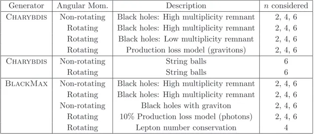
The canonical Monte Carlo generators for the production of black hole signals are
Charybdis 2.104 [
58
] and Blackmax 2.2.0 [
59
,
60
]. Both programs are able to simulate a
range of rotating and non-rotating black hole and string ball states, exploring the
theoreti-cal modelling uncertainties discussed in section
1
. A variety of potential black hole signals
simulated with both generators are used to illustrate possible black hole models. They are
described in detail below and summarised in table
1
. The shower evolution and
hadronisa-tion of all signal samples uses Pythia 8.165 [
61
], with the MSTW2008LO [
62
] PDF set
and the AU2 tune. The mass of the black hole is used as the factorisation and
renormal-isation scales. The detector response is simulated using the ATLAS fast simulation [
63
].
The benchmark event samples are generated for two, four and six extra dimensions.
Both Monte Carlo generators are able to include the effects of the black hole angular
momentum, with similar treatments of the Hawking evaporation. Moreover, they contain
complementary and different modelling options for the more uncertain decay phases. Both
generators model losses of mass and angular momentum in the production phase:
Charyb-dis uses a model based on the Yoshino-Rychkov bounds [
58
,
64
], favouring smaller losses of
mass and angular momentum in the form of gravitons, whereas Blackmax parameterises
the losses as fixed fractions of their initial-state values. For each generator, a benchmark
model including these loss models is used to investigate their effect. The Blackmax
sam-ple assumes a 10% loss into photon modes. Blackmax can also model graviton emission
in the non-rotating case, which is considered in another benchmark sample. The
mod-elling of the remnant phase can have large effects on the event multiplicity, and hence the
experimental signature. Blackmax uses a final-burst remnant model, which gives
low-JHEP08(2014)103
Generator
Angular Mom.
Description
n considered
Charybdis
Non-rotating
Black holes: High multiplicity remnant
2, 4, 6
Rotating
Black holes: High multiplicity remnant
2, 4, 6
Rotating
Black holes: Low multiplicity remnant
2, 4, 6
Rotating
Production loss model (gravitons)
2, 4, 6
Charybdis
Non-rotating
String balls
6
Rotating
String balls
6
BlackMax
Non-rotating
Black holes: High multiplicity remnant
2, 4, 6
Rotating
Black holes: High multiplicity remnant
2, 4, 6
Non-rotating
Black holes with graviton
2, 4, 6
Rotating
10% Production loss model (photons)
2, 4, 6
Rotating
Lepton number conservation
4
Table 1. Summary of the TeV-scale gravity benchmark models considered.
and high-multiplicity remnant decays, corresponding to fixed two-body decay, and variable
decay with a mean of four particles, respectively. The high-multiplicity options of both
gen-erators produce similar distributions of particle multiplicities and p
T. Baryon and lepton
numbers may not be conserved in black hole interactions [
65
,
66
]; however, both generators
conserve baryon number to avoid problems with colour in hadronisation. The default
gen-erator treatment is to violate lepton number, though both options are available. A
bench-mark sample with lepton number conservation is produced with Blackmax, for n = 4 only.
String ball samples are produced with Charybdis for both rotating and non-rotating cases,
six extra dimensions, a string coupling g
S= 0.4, and M
D= g
−2/(n+2)
S
M
S= 1.26 M
S.
For each benchmark model, samples are generated with M
Dvarying from 1.5 to 4 TeV
(M
Svarying from 1 to 3 TeV for string ball models) and M
thfrom 4–6.5 TeV, so as to cover
the production cross-sections to which the current data are sensitive. The productions
cross-sections are calculated by the event generators.
5
Object reconstruction
Jets are reconstructed using the anti-k
tjet clustering algorithm [
67
] with radius parameter
R = 0.4. The inputs to the jet algorithm are clusters seeded from calorimeter cells with
energy deposits significantly above the measured noise [
68
]. Jet energies are corrected [
69
]
for detector inhomogeneities, and the non-compensating response of the calorimeter, using
factors derived from test beam, cosmic ray and pp collision data, and from the full detector
simulation. Furthermore, jets are corrected for energy from additional pp collisions
(pile-up) using a method proposed in ref. [
70
], which estimates the pile-up activity in any given
event, as well as the sensitivity of any given jet to pile-up. Selected jets are required to have
p
T> 60 GeV and |η| < 2.8. Events containing jets failing to satisfy the quality criteria
that discriminate against electronic noise and non-collision backgrounds are rejected [
69
].
Electrons are reconstructed from clusters in the electromagnetic calorimeter associated
JHEP08(2014)103
electron identification criteria based on the calorimeter shower shape, track quality and
track matching with the calorimeter cluster are referred to as “medium” and “tight”, with
“tight” offering increased background rejection over “medium” in exchange for some loss
in identification efficiency. Electrons are required to have p
T> 60 GeV, |η| < 2.47 and
to satisfy the “medium” electron definition. Candidates in the transition region between
barrel and end-cap calorimeters, 1.37 < |η| < 1.52, are excluded. Electron candidates
are required to be isolated: the sum of the p
Tof tracks within a cone of size ∆R =
p(∆η)
2+ (∆φ)
2= 0.2 around the electron candidate is required to be less than 10% of
the electron p
T.
Muon tracks are reconstructed from track segments in the various layers of the muon
spectrometer and then matched to corresponding tracks in the inner detector [
72
]. In order
to ensure good p
Tresolution, muons are required to have at least three hits in each of the
layers of either the barrel or end-cap region of the MS, and at least one hit in two layers of
the trigger chambers. Muon candidates passing through known misaligned chambers are
rejected, and the difference between the independent momentum measurements obtained
from the ID and MS must not exceed five times the sum in quadrature of the uncertainties
of the two measurements. Each muon candidate is required to have a minimum number of
hits in each of the subsystems of the ID, and to have p
T> 60 GeV and |η| < 2.4. In order
to reject muons resulting from cosmic rays, requirements are placed on the distance of each
muon track from the primary vertex: |z
0| < 1 mm and |d
0| < 0.2 mm, where z
0and d
0are the impact parameters of each muon in the longitudinal direction and transverse plane,
respectively. To reduce the background from non-prompt sources such as heavy-flavour
decays, muons must be isolated: the p
Tsum of tracks within a cone of size ∆R = 0.3
around the muon candidate is required to be less than 5% of the muon p
T. Ambiguities
between the reconstructed jets and leptons are resolved by applying the following criteria:
jets within a distance of ∆R = 0.2 of an electron candidate are rejected; furthermore, any
lepton candidate with a distance ∆R < 0.4 to the closest remaining jet is discarded.
The signal selection places no requirement on whether or not selected jets originate
from the hadronisation of a b-quark (b-jets). However, b-jets are used in the definition of
control regions, either by requiring at least one b-tagged jet, or by vetoing any event with
at least one b-tagged jet. To identify b-jets, the employed algorithm [
73
] uses multivariate
techniques to combine information derived from tracks within jets, such as impact
parame-ters and reconstructed vertices displaced from the primary vertex. The efficiency of tagging
a b-jet in simulated t¯
t events is estimated to be 70%, with charm jet, light-quark jet and
τ lepton rejection factors of about 5, 147 and 13, respectively. Scale factors associated
with the identification efficiencies of b-jets are applied to bring the simulation into better
agreement with the data [
74
].
The missing transverse momentum ~
p
Tmiss, with its magnitude E
Tmiss, is defined as the
negative vectorial p
Tsum of reconstructed objects in the event, comprising selected
lep-tons, jets with p
T> 20 GeV, any additional non-isolated muons with p
T> 10 GeV, and
calorimeter clusters not belonging to any of the aforementioned object types [
75
]. E
Tmissis only used to define control regions for the background estimation and not to define the
JHEP08(2014)103
700 800 900 1000 1100 1200 1300 1400 1500 Events / 20 GeV 1 10 2 10 3 10 4 10 Data Total Background W+jets (SHERPA) Multi-jets (Matrix Method)*+jets (SHERPA) γ Z/ (POWHEG) t t
Single top (ACERMC/MCatNLO) Diboson (HERWIG) [GeV] T p
∑
700 800 900 1000 1100 1200 1300 1400 1500 Data / Bkg 0.60.8 1 1.2 1.4 ATLAS = 8 TeV s , -1 L dt = 20.3 fb∫
electron channel 700 800 900 1000 1100 1200 1300 1400 1500 Events / 20 GeV 1 10 2 10 3 10 4 10 Data Total Background W+jets (SHERPA) *+jets (SHERPA) γ Z/ (POWHEG) t tSingle top (ACERMC/MCatNLO) Diboson (HERWIG) [GeV] T p
∑
700 800 900 1000 1100 1200 1300 1400 1500 Data / Bkg 0.60.8 1 1.2 1.4 ATLAS = 8 TeV s , -1 L dt = 20.3 fb∫
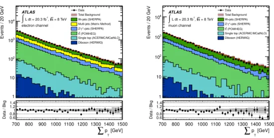
muon channelFigure 1. The P pT, after event preselection, in the electron (left) and muon (right) channels.
The Monte Carlo distributions are rescaled using scale factors derived in the appropriate control regions, as described in the text. The lower panels show the ratio of the data to the expected background, with the statistical uncertainty on data (points), and separately, the fractional total uncertainty on the background (shaded band).
is calculated from the lepton transverse momentum vector, ~
p
Tℓ, and the missing transverse
momentum vector ~
p
missT
:
m
T=
q
2 · p
ℓT
· E
Tmiss· (1 − cos(∆φ(~p
Tℓ, ~
p
Tmiss))) .
(5.1)
6
Event selection
The selected events contain at least one high-p
Tisolated lepton and at least two additional
objects (leptons and jets). Two statistically independent channels are defined, based on
whether the highest-p
Tlepton matching a lepton reconstructed by the trigger is an electron
or a muon. This lepton is called the “leading” lepton. For the electron channel, the leading
electron is required to pass the “tight” selection criteria. The muon channel has a lower
acceptance, due to the stringent hit requirements in the muon spectrometer.
The high multiplicity final states of interest are distinguished from SM background
events using the quantity:
X
p
T=
X
i=objects
p
T,iif p
T,i> 60 GeV,
(6.1)
the scalar sum of the transverse momenta of the selected leptons and jets with p
T> 60 GeV,
described in section
5
. Events with 700 GeV <
P p
T< 1500 GeV constitute a preselection
sample from which special control regions are defined by adding other selection criteria.
Figure
1
shows the
P p
Tdistribution for preselected events, for the electron and muon
channels. The signal, containing multiple high-p
Tleptons and jets, would manifest itself
JHEP08(2014)103
Quantity
Region
Sideband
Signal
P p
T1000–2000 GeV
> 2000 GeV
Object multiplicity
at least 3 objects above 100 GeV
Leading lepton
at least 1 lepton with p
T> 100 GeV
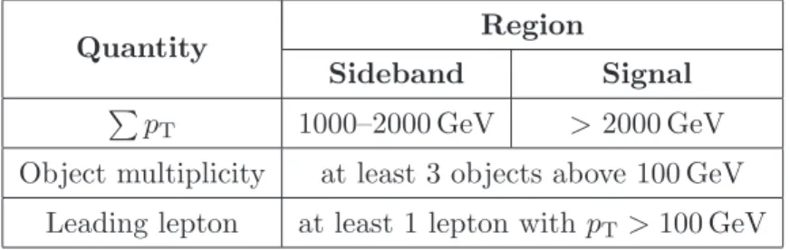
Table 2. Definitions of the sideband and signal regions.
For the signal region, in order to reduce the SM background contributions, events are
required to contain at least three reconstructed objects with p
T> 100 GeV, at least one
of which must be a lepton, as well as to have a
P p
Tof at least 2000 GeV. In each of the
channels, the signal region above
P p
T= 2000 GeV is divided into multiple slices, with
P p
Tthresholds increasing in steps of 200 GeV. This allows the analysis to be sensitive to
a wide range of signal models, and values of M
Dand M
th. Events in the range 1000 GeV
<
P p
T< 2000 GeV, but otherwise with the same requirements as the signal region,
constitute a “sideband” region. The contributions from signal models not yet excluded by
earlier analyses to the sideband region are well below 1%. The selection criteria for the
sideband and signal regions are summarised in table
2
.
7
Background estimation
The dominant sources of Standard Model background in this search are the production
of W and Z bosons in association with jets, t¯
t production and multi-jet processes. There
are three sources of leptons that can contribute to the background. Firstly, the leptonic
decays of W and Z bosons and top quarks produce events with real leptons, with associated
high-p
Tjets (hereinafter called “prompt” backgrounds). Secondly, leptons can arise from
semileptonic decays of heavy flavour hadrons. These are typically non-prompt and not
isolated. Thirdly, other objects such as jets can be misidentified.
The backgrounds are estimated using a combination of data-driven and MC-based
tech-niques. Prompt backgrounds are estimated using MC samples, normalised in data control
regions that are dominated by a single background component and kinematically close to
the signal region. The multi-jet contribution is estimated using a data-driven technique that
is more reliable than simulation for determining “fake” lepton backgrounds, due to its
inde-pendence from MC modelling uncertainties such as hadronisation and detector simulation.
At very high
P p
T, the number of events in the simulated samples becomes small,
and therefore subject to large statistical fluctuations. Therefore, for each background
component, the
P p
Tdistribution is fitted to a functional form to smooth the backgrounds
and extrapolate them to very high
P p
T.
7.1
Prompt background estimation from control regions
The background estimates for processes involving prompt leptons are based on MC
sim-ulations normalised in control regions, each dominated by a single process, as discussed
above. The normalisation factors are determined, separately for the electron and muon
JHEP08(2014)103
Quantity
Control Region
Z+jets
W +jets
t¯
t
P p
T700–1500 GeV
Object multiplicity
at least 3 objects (leptons or jets) with p
T> 60 GeV
Leading lepton
at least 1 lepton with p
T> 60 GeV
m
ℓℓ80–100 GeV
n/a
E
missT
n/a
> 60 GeV
n/a
Lepton multiplicity
exactly 2, opposite sign
exactly 1
same flavour
b-jet multiplicity
n/a
exactly 0
> 1
Jet multiplicity
n/a
> 3
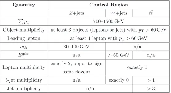
Table 3. Definitions of the SM background-dominated control regions. The first three rows repre-sent the preselection criteria.
channels, for the three main backgrounds: Z+jets, W +jets and t¯
t. The control regions are
defined in table
3
. For the Z+jets control region, events passing preselection requirements
are required to contain two electrons or muons of opposite charge and to have dilepton
in-variant mass between 80 GeV and 100 GeV. The W +jets control region consists of events
with exactly one lepton, no b-tagged jets and E
missT
greater than 60 GeV, where the last
two requirements help to reduce the t¯
t and Z+jets/multi-jet contributions, respectively.
The t¯
t control region consists of events with exactly one lepton and at least four jets, of
which at least two must be tagged as b-jets. The final criterion ensures no overlap with
the W +jet control region and preferentially selects for the top quark decays. The purities
of the Z+jets, W +jets and t¯
t control regions are estimated from Monte Carlo simulations
to be about 98%, 70% and 90%, respectively.
The number of events predicted by the MC simulation is compared to the observed
number of events in data in each of the control regions, to derive the scale factors used to
normalise the backgrounds. Due to non-negligible contamination by W +jets events in the
t¯
t control region and vice-versa, two coupled equations determine the two normalisations
that lead to agreement between data and MC simulation. The derived scale factors to
be applied to the background predictions in the electron (muon) channels are 1.00 (1.08)
for t¯
t, 0.76 (0.81) for W +jets, and 0.90 (0.93) for Z+jets. They are compatible between
channels within their statistical uncertainties.
The much smaller contributions from single-top and diboson processes are estimated
to comprise approximately 2% and 0.5%, respectively, of the events in the sideband and
signal regions. Their estimates are taken directly from Monte Carlo simulations.
Figure
2
shows the good agreement obtained in kinematic distributions in the
con-trol regions. The
P p
Tdistribution for each control region is shown in figure
3
, which
JHEP08(2014)103
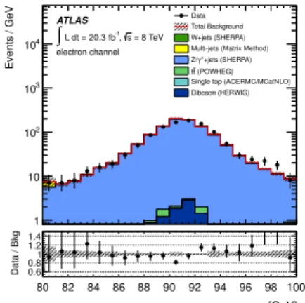
80 82 84 86 88 90 92 94 96 98 100 Events / GeV 1 10 2 10 3 10 4 10 Data Total Background W+jets (SHERPA) Multi-jets (Matrix Method)*+jets (SHERPA) γ Z/ (POWHEG) t t
Single top (ACERMC/MCatNLO) Diboson (HERWIG) [GeV] ll m 80 82 84 86 88 90 92 94 96 98 100 Data / Bkg 0.60.8 1 1.2 1.4 ATLAS = 8 TeV s , -1 L dt = 20.3 fb ∫ electron channel
(a) Z+jets CR, dilepton invariant mass, electron channel. 80 82 84 86 88 90 92 94 96 98 100 Events / GeV 1 10 2 10 3 10 4
10 DataTotal Background
W+jets (SHERPA) *+jets (SHERPA) γ Z/ (POWHEG) t t
Single top (ACERMC/MCatNLO) Diboson (HERWIG) [GeV] ll m 80 82 84 86 88 90 92 94 96 98 100 Data / Bkg 0.60.8 1 1.2 1.4 ATLAS = 8 TeV s , -1 L dt = 20.3 fb ∫ muon channel
(b) Z+jets CR, dilepton invariant mass, muon channel. 0 20 40 60 80 100 120 140 160 180 200 Events / 10 GeV 1 10 2 10 3 10 4 10 5 10 Data Total Background W+jets (SHERPA) Multi-jets (Matrix Method)
*+jets (SHERPA) γ Z/ (POWHEG) t t
Single top (ACERMC/MCatNLO) Diboson (HERWIG) [GeV] T Electron m 0 20 40 60 80 100 120 140 160 180 200 Data / Bkg 0.60.8 1 1.2 1.4 ATLAS = 8 TeV s , -1 L dt = 20.3 fb ∫ electron channel
(c) W +jets CR, mT, electron channel.
0 20 40 60 80 100 120 140 160 180 200 Events / 10 GeV 1 10 2 10 3 10 4 10 5 10 Data Total Background W+jets (SHERPA) *+jets (SHERPA) γ Z/ (POWHEG) t t
Single top (ACERMC/MCatNLO) Diboson (HERWIG) [GeV] T Muon m 0 20 40 60 80 100 120 140 160 180 200 Data / Bkg 0.60.8 1 1.2 1.4 ATLAS = 8 TeV s , -1 L dt = 20.3 fb ∫ muon channel
(d) W +jets CR, mT, muon channel.
4 5 6 7 8 9 10 Events 1 10 2 10 3 10 4 10 5
10 DataTotal Background
W+jets (SHERPA) Multi-jets (Matrix Method)
*+jets (SHERPA) γ Z/ (POWHEG) t t
Single top (ACERMC/MCatNLO) Diboson (HERWIG) [GeV] >60 GeV T p nJets 4 5 6 7 8 9 Data / Bkg 0.60.8 1 1.2 1.4 ATLAS = 8 TeV s , -1 L dt = 20.3 fb ∫ electron channel
(e) t¯t CR, jet multiplicity, electron channel. 4 5 6 7 8 9 10 Events 1 10 2 10 3 10 4 10 5 10 Data Total Background W+jets (SHERPA) *+jets (SHERPA) γ Z/ (POWHEG) t t
Single top (ACERMC/MCatNLO) Diboson (HERWIG) [GeV] >60 GeV T p nJets 4 5 6 7 8 9 Data / Bkg 0.60.8 1 1.2 1.4 ATLAS = 8 TeV s , -1 L dt = 20.3 fb ∫ muon channel
(f) t¯t CR, jet multiplicity, muon channel.
Figure 2. Kinematic distributions for the three control regions (CR). The Monte Carlo samples are normalised to data using scale factors, according to the method described in section 7. The regions are defined in table 3. Some background contributions are very small in specific control regions. The lower panels show the ratio of the data to the expected background, with the statistical uncertainty on data (points), and separately, the fractional total uncertainty on the background (shaded band).
JHEP08(2014)103
700 800 900 1000 1100 1200 1300 1400 1500 Events / 50 GeV 1 10 2 10 3 10 Data Total Background W+jets (SHERPA) Multi-jets (Matrix Method)*+jets (SHERPA) γ Z/ (POWHEG) t t
Single top (ACERMC/MCatNLO) Diboson (HERWIG) [GeV] T p ∑ 700 800 900 1000 1100 1200 1300 1400 1500 Data / Bkg 0.60.8 1 1.2 1.4 ATLAS = 8 TeV s , -1 L dt = 20.3 fb ∫ electron channel
(a) Z+jets CR,PpT, electron channel.
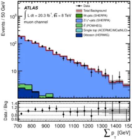
700 800 900 1000 1100 1200 1300 1400 1500 Events / 50 GeV 10 2 10 3 10 Data Total Background W+jets (SHERPA) *+jets (SHERPA) γ Z/ (POWHEG) t t
Single top (ACERMC/MCatNLO) Diboson (HERWIG) [GeV] T p ∑ 700 800 900 1000 1100 1200 1300 1400 1500 Data / Bkg 0.60.8 1 1.2 1.4 ATLAS = 8 TeV s , -1 L dt = 20.3 fb ∫ muon channel
(b) Z+jets CR,PpT, muon channel.
700 800 900 1000 1100 1200 1300 1400 1500 Events / 50 GeV 1 10 2 10 3 10 4 10 Data Total Background W+jets (SHERPA) Multi-jets (Matrix Method)
*+jets (SHERPA) γ Z/ (POWHEG) t t
Single top (ACERMC/MCatNLO) Diboson (HERWIG) [GeV] T p ∑ 700 800 900 1000 1100 1200 1300 1400 1500 Data / Bkg 0.60.8 1 1.2 1.4 ATLAS = 8 TeV s , -1 L dt = 20.3 fb ∫ electron channel
(c) W +jets CR,PpT, electron channel.
700 800 900 1000 1100 1200 1300 1400 1500 Events / 50 GeV 1 10 2 10 3 10 4
10 DataTotal Background
W+jets (SHERPA) *+jets (SHERPA) γ Z/ (POWHEG) t t
Single top (ACERMC/MCatNLO) Diboson (HERWIG) [GeV] T p ∑ 700 800 900 1000 1100 1200 1300 1400 1500 Data / Bkg 0.60.8 1 1.2 1.4 ATLAS = 8 TeV s , -1 L dt = 20.3 fb ∫ muon channel
(d) W +jets CR,PpT, muon channel
700 800 900 1000 1100 1200 1300 1400 1500 Events / 50 GeV 1 10 2 10 3 10 Data Total Background W+jets (SHERPA) Multi-jets (Matrix Method)
*+jets (SHERPA) γ Z/ (POWHEG) t t
Single top (ACERMC/MCatNLO) Diboson (HERWIG) [GeV] T p ∑ 700 800 900 1000 1100 1200 1300 1400 1500 Data / Bkg 0.60.8 1 1.2 1.4 ATLAS = 8 TeV s , -1 L dt = 20.3 fb ∫ electron channel
(e) t¯t CR,PpT, electron channel
700 800 900 1000 1100 1200 1300 1400 1500 Events / 50 GeV 1 10 2 10 3 10 Data Total Background W+jets (SHERPA) *+jets (SHERPA) γ Z/ (POWHEG) t t
Single top (ACERMC/MCatNLO) Diboson (HERWIG) [GeV] T p ∑ 700 800 900 1000 1100 1200 1300 1400 1500 Data / Bkg 0.60.8 1 1.2 1.4 ATLAS = 8 TeV s , -1 L dt = 20.3 fb ∫ muon channel (f) t¯t CR,PpT, muon channel.
Figure 3. P pTdistributions for each control region (CR). The Monte Carlo samples are normalised
to data using scale factors, according to the method described in section7. The regions are defined in table 3. Some background contributions are very small in specific control regions. The lower panels show the ratio of the data to the expected background, with the statistical uncertainty on data (points), and separately, the fractional total uncertainty on the background (shaded band). .
JHEP08(2014)103
7.2
Backgrounds from misidentified objects and non-prompt leptons
The backgrounds from misidentified objects and non-prompt leptons are estimated with
a data-driven matrix method, described in detail in ref. [
76
]. In the electron channel,
this contribution is dominated by the misidentification of hadronic jets, resulting in “fake”
electrons. In order to make an estimate using this method, a sample enriched in multi-jet
events is obtained by relaxing the electron selection criteria so as to increase the
contribu-tion from fakes. This is achieved by loosening the leading electron identificacontribu-tion criteria
from “tight” to “medium”. The contribution from two or more fake electrons is found to
be negligible.
The numbers of data events in the sample which pass (N
pass) and fail (N
fail) the
nominal tighter lepton selection requirements are counted. Defining N
promptand N
fakeas
the numbers of events for which the leptons are prompt and fake, respectively, the following
relationships hold:
N
pass= ǫ
promptN
prompt+ ǫ
fakeN
fake,
(7.1)
and
N
fail= (1 − ǫ
prompt)N
prompt+ (1 − ǫ
fake)N
fake,
(7.2)
where ǫ
promptand ǫ
fakeare the relative efficiencies for prompt and fake leptons to pass the
nominal selection, given that they satisfy the looser selection criteria. The simultaneous
solution of these two equations gives a prediction for the number of events in data with
fake leptons satisfying the nominal criteria, taken to be the estimated number of multi-jet
events:
N
fake=
N
fail− (1/ǫ
prompt− 1)N
pass1 − ǫ
fake/ǫ
prompt.
(7.3)
The efficiencies ǫ
promptand ǫ
fakeare determined from control regions enriched in
prompt-lepton or fake-lepton events, respectively. A fake-enhanced control sample is
ob-tained starting from the preselection region, selecting events with exactly one lepton that
satisfies the relaxed lepton criteria described above, m
T< 40 GeV and m
T+ E
Tmiss<
60 GeV. No
P p
Tdependence in ǫ
fakeand ǫ
promptis observed, and the minimum
P p
Trequirement for these regions is set to 500 GeV, compared with
P p
T> 700 GeV for the
other control regions, in order to gain statistical power.
The efficiency for identifying fakes as prompt leptons is given by the fraction of the
events in this control region that also pass the nominal lepton selection, after subtracting,
in both instances, the estimated contribution from prompt-lepton backgrounds (derived
from MC simulations, renormalised to match data in control regions, as described above).
For the electron channel, some dependence on the p
Tand η of the leading electron is
observed, which is taken into account by using p
T- and η-dependent ǫ
fake; they vary in the
range 0.26–0.42.
An equivalent procedure is followed for the muon channel, where the dominant
contri-bution arises from non-prompt muons resulting from semileptonic decays, usually of heavy
flavour. An event sample enhanced in these is formed by removing both the jet-muon
JHEP08(2014)103
be negligibly small, consistent with zero: 0.0043 ± 0.0040 (stat), or < 0.011 at 95% CL;
the resultant predicted background is negligible.
The efficiency ǫ
promptis evaluated in a region with the same selection as the Z+jets
control region, except for the relaxed
P p
Trequirement, 500 GeV <
P p
T< 1500 GeV,
to match that used in the control region for fake and non-prompt leptons. The relative
efficiency for identifying prompt leptons is obtained through the ratio of the number of
events in which both leptons pass the nominal selection to those in which only one does.
The measured values of ǫ
promptare 0.960 ±0.007 and 0.942±0.007 for electrons and muons,
respectively, where the quoted uncertainties are statistical only.
7.3
Background smoothing with fits
At high
P p
T, particularly beyond
P p
T≈ 3500 GeV, the numbers of events in the
simu-lated background samples are small and consequently have large statistical uncertainties.
To provide a more robust prediction in the signal region, the
P p
Tdistributions of each
in-dividual background are fitted to an empirical function that enables the background shape
to be smoothed and extended without being strongly affected by statistical fluctuations.
This method reduces the statistical uncertainty, by using information at lower
P p
Tto
constrain the shape of the distribution, but introduces systematic uncertainties from the
choice of binning and normalisation region, and from the choice of fit function. These are
further discussed in section
8
. The fit function used is given by:
F = (1 − x)
p0x
p1x
p2log(x),
(7.4)
where x =
P p
T/
√
s, and p
0, p
1and p
2are the parameters to be fitted. The overall
normalisation is fixed by a combination of p
0, p
1and p
2. The function was chosen for
its stable and reliable description of the shape of the distributions over the full range
of
P p
T. In previous studies [
77
–
79
], ATLAS and other experiments have found that
this ansatz provides satisfactory fits to kinematic distributions. The fit range begins at
P p
T= 700 GeV, and ends where the number of simulated events in a given bin is below
five. The start- and end-points of the fit range, as well as the binning, are varied, and the
results are consistent with the nominal fit within the statistical uncertainty. Although the
default fits (shown in figures
4
and
5
) are of high quality and stability, there is an uncertainty
associated with the choice of background fit function. To assess this, an alternative function
was chosen that succeeds in describing the distributions at low and intermediate
P p
Tbut
has a different shape than the nominal function at high
P p
T, where the numbers of
simulated events are smaller. This function is given by:
F
alt=
p
0x
(1 − p
1x)
p2
,
(7.5)
where x =
P p
T/
√
s, and p
0, p
1and p
2are the parameters to be fitted.
In the bins where the prediction from this alternative function falls outside the
nom-inal fit uncertainty, the difference between the nomnom-inal and alternative functions is used
as the fit uncertainty, i.e. an envelope of them is taken and symmetrised, to be
conserva-tive, ensuring that the total fit uncertainty covers alternative functions and the inherent
uncertainty of the fit itself.
JHEP08(2014)103
The
P p
Tdistributions for each MC-simulated prompt-lepton background are
dis-played in figure
4
; the curves shown represent the results of the binned maximum likelihood
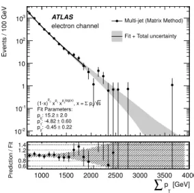
fits. The multi-jet background in the electron channel estimated from data is fitted to the
same function, as shown in figure
5
. The fit quality is high, with typical χ
2/d.o.f. values
between 0.9 and 1.6.
The fitted shapes of the individual backgrounds are combined according to their relative
predicted contributions (as discussed in the preceding sections, computed in a subset of
the sideband region, 1000 <
P p
T< 1500 GeV) to give an overall background template
shape. In order to reduce the systematic uncertainty, this is normalised to data in this
same region by a minimisation of the χ
2difference between the data and the background
template. This results in a normalisation consistent with that determined from the control
regions within the 4% uncertainty resulting from the statistical uncertainty on the data in
these bins. The resulting background estimate gives a smooth and stable prediction at all
values of
P p
T.
8
Systematic uncertainties
Sources of systematic uncertainty in the background prediction are taken into account.
These are reduced by the normalisation to data in the control regions, making the analysis
insensitive to
P p
T-independent uncertainties, such as those on the luminosity
measure-ment (this uncertainty is applied to the signal expectation). Uncertainties on the shape of
the
P p
Tdistribution, on the other hand, can have an impact on the background prediction.
The uncertainty from the fit to the backgrounds is the dominant systematic uncertainty.
Its impact on the background yield varies from 25% (20%) for the
P p
T> 2000 GeV region,
to 140% (190%) for the
P p
T> 3200 GeV region, for the electron (muon) channel. The
systematic uncertainties resulting from variations of the fit range and alternative choices
for the
P p
Tregion used to normalise the background template are found to be negligible.
The experimental uncertainties are small compared to the fit uncertainty in all signal
regions considered. Their impact is assessed by applying each systematic uncertainty to
the background samples, changing both the relative fractions of the backgrounds and their
shapes. This is then propagated to the fits, and a new spectrum is obtained. The
dif-ference between the nominal prediction and the new prediction determines the systematic
uncertainty. The most important experimental systematic uncertainty comes from the jet
energy scale. This is determined using in situ techniques [
69
], and gives rise to
system-atic uncertainties of 2–10% for the lower
P p
Tsignal regions, and no more than 20% for
the highest
P p
Tsignal regions. Systematic uncertainties from jet energy resolution and
b-tagging [
73
,
80
] are found to be small (< 5%), even for the highest
P p
Tthresholds
con-sidered, while uncertainties from missing transverse energy, and lepton scale, identification
and resolution are found to be completely negligible. Additional uncertainties arise from
the choice of MC generators (5–10%, comparing the nominal generators for the three main
prompt backgrounds with Alpgen) and limited knowledge about the parton distribution
functions at high
P p
T(2–10%). The latter includes both the appropriate PDF error set
JHEP08(2014)103
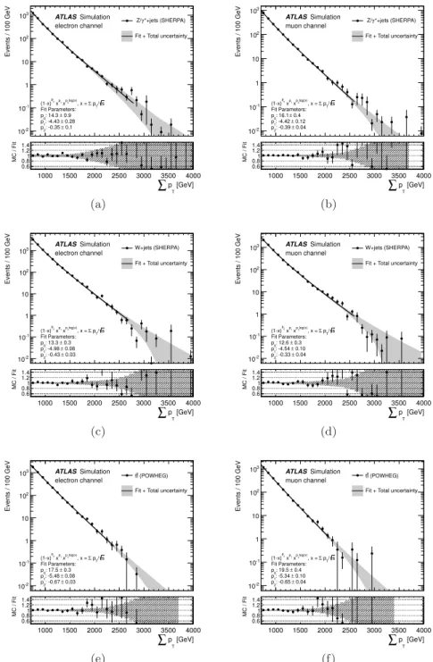
Events / 100 GeV -2 10 -1 10 1 10 2 10 3 10 *+jets (SHERPA) γ Z/Fit + Total uncertainty
[GeV] T p ∑ 1000 1500 2000 2500 3000 3500 4000 MC / Fit 0.6 0.81 1.2 1.4 ATLAS Simulation electron channel s / T p Σ , x = log(x) 2 p x 1 p x 0 p (1-x) Fit Parameters: 0.9 ± : 14.3 0 p 0.28 ± : -4.43 1 p 0.1 ± : -0.35 2 p (a) Events / 100 GeV -2 10 -1 10 1 10 2 10 3 10 *+jets (SHERPA) γ Z/
Fit + Total uncertainty
[GeV] T p ∑ 1000 1500 2000 2500 3000 3500 4000 MC / Fit 0.6 0.81 1.2 1.4 ATLAS Simulation muon channel s / T p Σ , x = log(x) 2 p x 1 p x 0 p (1-x) Fit Parameters: 0.4 ± : 16.1 0 p 0.12 ± : -4.42 1 p 0.04 ± : -0.39 2 p (b) Events / 100 GeV -2 10 -1 10 1 10 2 10 3 10 W+jets (SHERPA)
Fit + Total uncertainty
[GeV] T p ∑ 1000 1500 2000 2500 3000 3500 4000 MC / Fit 0.6 0.81 1.2 1.4 ATLAS Simulation electron channel s / T p Σ , x = log(x) 2 p x 1 p x 0 p (1-x) Fit Parameters: 0.3 ± : 13.3 0 p 0.08 ± : -4.98 1 p 0.03 ± : -0.43 2 p (c) Events / 100 GeV -2 10 -1 10 1 10 2 10 3 10 W+jets (SHERPA) Fit + Total uncertainty
[GeV] T p ∑ 1000 1500 2000 2500 3000 3500 4000 MC / Fit 0.6 0.81 1.2 1.4 ATLAS Simulation muon channel s / T p Σ , x = log(x) 2 p x 1 p x 0 p (1-x) Fit Parameters: 0.3 ± : 12.6 0 p 0.10 ± : -4.54 1 p 0.04 ± : -0.33 2 p (d) Events / 100 GeV -2 10 -1 10 1 10 2 10 3 10 tt (POWHEG) Fit + Total uncertainty
[GeV] T p ∑ 1000 1500 2000 2500 3000 3500 4000 MC / Fit 0.6 0.81 1.2 1.4 ATLAS Simulation electron channel s / T p Σ , x = log(x) 2 p x 1 p x 0 p (1-x) Fit Parameters: 0.3 ± : 17.5 0 p 0.08 ± : -5.48 1 p 0.03 ± : -0.67 2 p (e) Events / 100 GeV -2 10 -1 10 1 10 2 10 3 10 (POWHEG) tt
Fit + Total uncertainty
[GeV] T p ∑ 1000 1500 2000 2500 3000 3500 4000 MC / Fit 0.6 0.81 1.2 1.4 ATLAS Simulation muon channel s / T p Σ , x = log(x) 2 p x 1 p x 0 p (1-x) Fit Parameters: 0.4 ± : 19.5 0 p 0.10 ± : -5.34 1 p 0.04 ± : -0.65 2 p (f)
Figure 4. The P pT distributions and fit curves for (a, b) Z+jets; (c, d) W +jets (+ diboson);
and (e, f) t¯t (+ single-top) MC-simulated events. Distributions for the electron channel are on the left while those for the muon channel are on the right. The shaded bands on the fit curves reflect the total uncertainty on the fit, including the systematic uncertainty discussed in section7.3. The length of the black line indicates theP pTrange fitted. The lower panels show the ratio of the MC
prediction to the fit, with the statistical uncertainty on the MC prediction (points), and separately, the fractional uncertainty on the fit (shaded band).
JHEP08(2014)103
Events / 100 GeV -2 10 -1 10 1 10 2 10 310 Multi-jet (Matrix Method) Fit + Total uncertainty
[GeV] T p
∑
1000 1500 2000 2500 3000 3500 4000 Prediction / Fit 0.6 0.81 1.2 1.4 ATLAS electron channel s / T p Σ , x = log(x) 2 p x 1 p x 0 p (1-x) Fit Parameters: 2.0 ± : 15.2 0 p 0.60 ± : -4.82 1 p 0.22 ± : -0.45 2 pFigure 5. TheP pTdistribution and fit curve for the multi-jet background in the electron channel.
The shaded band on the fit curve reflects the total uncertainty on the fit, including the systematic uncertainty discussed in section7.3. The length of the black line indicates the P pT range fitted.
The lower panel shows the ratio of the matrix method’s prediction to the fit, with the statistical uncertainty on the matrix method’s prediction (points), and separately, the fractional uncertainty on the fit (shaded band).
with MSTW2008nlo. Uncertainties from the choice of hadronisation and factorisation
scales were considered and found to be negligible.
Uncertainties on the signal yields include the detector response uncertainties discussed
above, luminosity and statistical uncertainties. Uncertainties that affect both the
back-ground and the signal are taken to be completely correlated. In addition, a 5% systematic
uncertainty is included on the signal normalisation, corresponding to the maximum
ob-served acceptance difference between MC-simulated samples using full GEANT4
simula-tion and the fast simulasimula-tion. The effect of PDF variasimula-tions on the signal acceptance is found
to be negligible. The theoretical and modelling uncertainties on these states motivate the
choice of benchmark models and are discussed in section
4
; limits are set for exactly these
benchmark models.
9
Results and interpretation
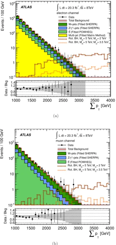
The
P p
Tdistributions observed from data and predicted from SM processes for the
elec-tron and muon channels in the sideband and signal regions are given in figure
6
, with two
representative signal distributions superimposed: rotating black holes with n = 6 and M
th= 5 TeV, one with M
D= 2 TeV, the other with M
D= 3.5 TeV.
5The yields in the signal
region for various choices of
P p
Tthreshold are shown in table
4
. In both channels, the
fraction of the W +jets background, already dominant at lower
P p
T, increases further for
higher
P p
T. The W +jets background constitutes 45% (66%) of the background yield
above
P p
T= 2000 GeV in the electron (muon) channel; the contribution from Z+jets is
JHEP08(2014)103
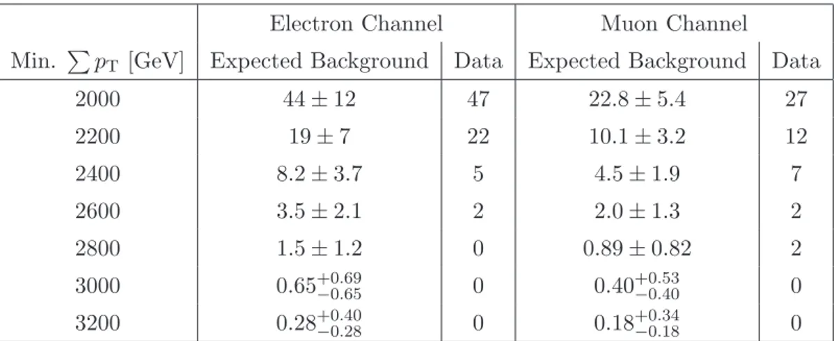
Electron Channel
Muon Channel
Min.
P p
T[GeV]
Expected Background
Data
Expected Background
Data
2000
44 ± 12
47
22.8 ± 5.4
27
2200
19 ± 7
22
10.1 ± 3.2
12
2400
8.2 ± 3.7
5
4.5 ± 1.9
7
2600
3.5 ± 2.1
2
2.0 ± 1.3
2
2800
1.5 ± 1.2
0
0.89 ± 0.82
2
3000
0.65
+0.69−0.650
0.40
+0.53 −0.400
3200
0.28
+0.40−0.280
0.18
+0.34 −0.180
Table 4. Expected SM background and observed event yields for the electron and muon channels, for the signal regions of this search. The quoted uncertainties on the background yields are the combined statistical and systematic uncertainties.
19% (17%), whereas t¯
t accounts for 15% (17%), with the remainder in the electron channel
being multi-jet events. For both channels, no data events are observed above
P p
T=
3000 GeV, in agreement with the background estimate.
No significant excess is observed beyond the Standard Model expectation for all choices
of
P p
Tthreshold: pvalues for the backgroundonly hypothesis are in the range 0.2
-0.5.
6Consequently, limits are set on the fiducial cross-section and on TeV-scale gravity
benchmark models, using the modified frequentist CL
sprescription described in ref. [
81
].
It compares the number of observed events in data with the SM expectation, using the
profile likelihood ratio as test statistic. All systematic uncertainties and their correlations
are taken into account via nuisance parameters.
Limits on the fiducial cross-section σ
fidpp→ℓX, defined as that part of the total
cross-section which is within the kinematic limits of the measurement, are calculated at 95% CL.
This requires the determination of a reconstruction efficiency factor, C
pp→ℓX, that converts
the observed signal yield (N
signal) to the yield in the fiducial region at the generator level:
σ
fidpp→ℓX=
N
signalL · C
pp→ℓX,
(9.1)
where L is the integrated luminosity used in the analysis.
The fiducial regions at generator level
7for the electron and muon channels are
de-fined from the simulated Charybdis signal events with final states that pass the following
requirements: the leading lepton is a prompt electron or muon
8within the experimental
acceptance, with p
T> 100 GeV and separated from jets with p
T> 60 GeV by ∆R(lepton,
jet) > 0.4; there are at least two additional jets or leptons with p
T> 100 GeV present in
6The p-value is truncated at 0.5, since only upward fluctuations of the background are taken into account. 7This includes parton showering and jet clustering, using the anti-k
t algorithm with R = 0.4 on stable
particles.
8Electrons and muons originating from τ leptons, heavy gauge bosons or directly from the black hole
JHEP08(2014)103
Events / 100 GeV -1 10 1 10 2 10 3 10 4 10 Data Total Background W+jets (Fitted SHERPA)*+jets (Fitted SHERPA)
γ
Z/
(Fitted POWHEG) tt
Multi-jet (Fitted Matrix Method) = 2 TeV D = 5 TeV, M th Rot. BH, M = 3.5 TeV D = 5 TeV, M th Rot. BH, M [GeV] T p
∑
1000 1500 2000 2500 3000 3500 4000 Data / Bkg 0.60.8 1 1.2 1.4 ATLAS∫
L dt = 20.3 fb-1, s = 8TeV electron channel (a) Events / 100 GeV -1 10 1 10 2 10 3 10 Data Total Background W+jets (Fitted SHERPA)*+jets (Fitted SHERPA)
γ Z/ (Fitted POWHEG) tt = 2 TeV D = 5 TeV, M th Rot. BH, M = 3.5 TeV D = 5 TeV, M th Rot. BH, M [GeV] T p
∑
1000 1500 2000 2500 3000 3500 4000 Data / Bkg 0.60.8 1 1.2 1.4 ATLAS∫
L dt = 20.3 fb-1, s = 8TeV muon channel (b)Figure 6. TheP pTdistributions in the (a) electron and (b) muon channels. Two representative
signal distributions for rotating black holes with n = 6 are overlaid to illustrate the signal properties. The lower panels show the ratio of the data to the expected background, with the statistical uncertainty on data (points), and separately, the fractional total uncertainty on the background (shaded band).
JHEP08(2014)103
threshold [GeV] T p Σ 2000 2500 3000 3500 [fb] fid lX → pp σ 0 1 2 3 4 5 6 ATLAS = 8 TeV s , -1 L dt = 20.3 fb∫
95% CL Upper LimitObservedExpected
σ
1
±
Exp
Figure 7. Upper limits on the fiducial cross-sections σfid
pp→ℓX for the production of final states with
at least three objects passing a 100 GeV pT requirement including at least one lepton, and P pT
above threshold, for all final states with at least one electron or muon. The observed and expected 95% CL limits according to the CLs prescription are shown, as well as the ±1σ bounds on the
expected limit.
the event, and
P p
Tis above the signal region threshold. The requirements are summarised
in table
5
. Additionally, given the appropriate C
pp→ℓX, the channels can be combined to
set a limit on σ
fidpp→ℓX
for anomalous production of final states with a lepton (e or µ). In
this “lepton” channel limit, the expectations of the two channels are summed, with the
uncertainties combined, taking their correlations into account. For the wide range of
mod-els considered (black hole states, string ball states, rotating and non-rotating, low- and
high-multiplicity remnant states, etc.), C
pp→ℓXvaries from 47% to 82% (22% to 46%) for
the electron (muon) channel, and 34–64% for the combined case. It is lowest for two extra
dimensions, due to the lower multiplicity of the final state. The fiducial cross-section limits
are given in table
6
, where the lowest overall values of C
pp→ℓXwithin the range of the
model dependence are used (which correspond to n = 2). Figure
7
shows the limits on
σ
pp→ℓXfidfor the combined channels using this most conservative value of C
pp→ℓX.
Exclusion contours are obtained in the plane of M
Dand M
thfor several benchmark
models. In each of the channels, the signal region above
P p
T= 2000 GeV is divided
into multiple slices, with
P p
Tthresholds increasing in steps of 200 GeV. This allows the
analysis to be sensitive across a wider range of signal models, and values of M
Dand M
th.
For each point in the M
D-M
thplane, the
P p
Tslice that gives the best expected
limit is used.
9The resulting exclusions for the statistical combination of the electron and
muon channels, for benchmark black hole models simulated with Charybdis, for two, four
and six extra dimensions, are shown in figure
8
. The exclusions tend to be stronger for
higher n, due to the larger signal cross-sections. They also tend to be stronger for the
non-rotating case than for the rotating case, due to a larger number of Hawking emissions
JHEP08(2014)103
[TeV] D M 1.5 2 2.5 3 3.5 4 [TeV]th M 4.6 4.8 5 5.2 5.4 5.6 5.8 6 6.2 6.4 ATLAS = 8 TeV s , -1 L dt = 20.3 fb∫
Non-rotating Black Holes, CHARYBDIS
D / M th k = M Observed (n=2) Expected (n=2) Observed (n=4) Expected (n=4) Observed (n=6) Expected (n=6) (n=6) σ 1 ± Exp k=4 k=3 k=2 (a) [TeV] D M 1.5 2 2.5 3 3.5 4 [TeV]th M 4.6 4.8 5 5.2 5.4 5.6 5.8 6 6.2 6.4 ATLAS = 8 TeV s , -1 L dt = 20.3 fb
∫
Rotating Black Holes, CHARYBDIS
D / M th k = M Observed (n=2) Expected (n=2) Observed (n=4) Expected (n=4) Observed (n=6) Expected (n=6) (n=6) σ 1 ± Exp k=4 k=3 k=2 (b) [TeV] D M 1.5 2 2.5 3 3.5 4 [TeV] th M 4.6 4.8 5 5.2 5.4 5.6 5.8 6 6.2 6.4 ATLAS = 8 TeV s , -1 L dt = 20.3 fb
∫
Rotating Black Holes, low mult. remnant, CHARYBDIS
D / M th k = M Observed (n=2) Expected (n=2) Observed (n=4) Expected (n=4) Observed (n=6) Expected (n=6) (n=6) σ 1 ± Exp k=4 k=3 k=2 (c) [TeV] D M 1.5 2 2.5 3 3.5 4 [TeV] th M 4.6 4.8 5 5.2 5.4 5.6 5.8 6 6.2 6.4 ATLAS = 8 TeV s , -1 L dt = 20.3 fb
∫
Rotating Black Holes, Production losses, CHARYBDIS
D / M th k = M Observed (n=2) Expected (n=2) Observed (n=4) Expected (n=4) Observed (n=6) Expected (n=6) (n=6) σ 1 ± Exp k=4 k=3 k=2 (d)
Figure 8. The exclusion limits in the Mth–MDplane, with electron and muon channels combined,
for (a) non-rotating and (b) rotating black hole models in two, four and six extra dimensions, simulated with Charybdis. The lower panes show limits for (c) rotating black holes with low multiplicity remnant decays and (d) with production phase losses turned on. The solid (dashed) lines show the observed (expected) 95% CL limits, with the shaded band illustrating the expected ± 1 σ variation of the n = 6 expected limits. The ±1σ variation is comparable for the n = 2 and n = 4 models. Masses below the corresponding lines are excluded. The lighter grey lines indicate constant k = Mth/MD.