Multivariate interpolation model to estirnate the effort component of software projects

(1)

Information Technology Jowna1 5 (6): 1143-1145, 2006 ISSN 1812-5638

Multivariate Interpolation Model to Estirnate the

Effort Component of Software Projects

Mitat Uysal

Department of Computer Engineering,

Dogus University-Kadiköy-Acibadem, Istanbul, Turkey

Abstract: In this study, a multivariate interpolation model was develüped to estimate the effort component in the software projeets. The data set that was used consİsts of two independent variables, first İs Develüped Lines (DL) and second is Methodology (ME) and one dependent Variable Effort (E). The data set is taken from (Shin and Goel, 2000) and the results that are obtained İn my work are compared with the results of Shin and Goe1 ( 2001) that are produced using a different model based on RBF.

Key words: Software engineering, software eost estimation, multivariate interpolation, data analysis, curve fitting

INTRODUCTION

Estimation of resources, eost and schedule for a software development effort requires experience, access to good historical information and the courage to commit to quantitative measures when qualitative data are all that exist (Pressman, 1992).

The importance of software cost estirnation is well documented. Good estimation techniques serve as a basis for commlUlication between software personnel and non-software personnel such as managers, sales people or even customers (Knafe, 1995) .

As estirnation model for computer software uses empirically derived formulas to predict data that are a required part of the software project planning step (Pressman, 1992).

Resource models consist of one or more empirically derived equatiollS that predict effort (in person-months), project duration (in chronological months), or the other pertinent project data.

Basili (1980) described four classes of resources models:

• Static single-variable models • Static multi-variable models • Dynarnic multi-variable models • Theoretical models

The static single-variable model takes the form: Resources=Cı *

(Estİmated characteristİcs )C2

where the resources could be effort, project duration, staff size or requisite lines of software documentation. The constants Cı and C2 are derived from data collected from past projects. The basic version of the Constructive Cost Model or COCOMO is an example of a static single variable modeL.

Static multi-variable model has the following form: Resources = Cı ı eı + C2ı e2 + .

where eı is the ith software characteristics and C2b C22 are empirically derived constants for the ith characteristics (Pressmarm, 1992)

A dynamic multivariate model projects resource requirements as a flUlction of time.

A theoretical approach to dynamic multivariable modeling hypothesizes a continuous resource expenditure curve and from it, derives equatiollS that model the behavior of the resource. The Putnam Estimation Model is a theoretical dynarnic multi-variable modeL. Some new models are proposed for software cost estimation. One of them is Peters and Ramanna Model based on an application of the Choquet integral (Peters and Rammana, 1 996)

This is a form of multi-criteria decision-making where the numeric value computed by the Choquet integral is an expression of the degree of preference of one technology over another in developing a software system.

Neural Networks are another tool to develop software cost estirnation models. Idri

et al.

( 2002) proposed a new model for this. They have used the full purpose COCOMA '81 dataset to train and to test the network. The obtained accuracy of the network was acceptable.

(2)

Inform. TechnoZ. J

.• 5 (6): 1143-1145. 2006

SOFTWARE COST MODEL THAT IS USED IN TIDS WORK

The following software eost model İs used in present study:

Where E İs effort, DL İs Develüped Lines and

1.1E

İs methodology used İn the software project. f İs a nonıınear fwıction İn terrns ofDL and

1.1E.

Multivariate interpolation method was used to [ind the interpolated values of DL and

1.1E

using a data set that contaİns E, DL and

1.1E

values obtained from past projects. This data set is taken from (Shin and Goel. 2000) .

TWO DIMENSIONAL INTERPOLATION

The two dimensİonal flUletion table İs an array of [wıctiona! values f;,j = feDLi,

1.1E)

on a rectangular grid,

(DL,. ME,) as shown in Fig. 1.

Double lagrange interpolation İs to apply the lagrange interpolation method twice İn two dimensİollS (Nakamura. 2002). Therefore. the interpolation uses all the data points İn the table. Suppose the fwıction table has M colurnns and N rows. The coordinates of the points are denoted by (DLM. MEN) and the functioml

values by fm,n' Then, double Lagrange interpolation is given by

g(DL.ME) M N

LL

<Pm (DL)'I'" (ME)fm" m=l n=l

Where <Pm and lfn are shape flUletions given by

ME-ı+1

•

ME, ME,DL

ME, .•

DLı-ı DI., Fig. 1: Rectangular grid

Recoginze that <l>mCDL) 'I'"(ME) is a lwo dimensioml shape flUletion that beeomes zero at all the data points except at (DLm. ME").

SIMULATION RESUL TS

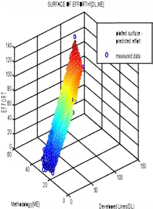
Applying the lwo variables (DL and ME) model mentioned above, the effort model surfaee as a flUletion ofDL and

1.1E

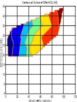
was obtained as shown Fig. 2.

In Fig. 3. the contours of the E � f(DL. ME) surface

are S hOWIl.

From these figures, we can note that the effort values are inereasing as DL inereases. AIso, there is a slight deerease in estimated effort with inereasing values of methodology. Both of these trends are similar to the results of Shin and Goel's who obtained the same figures

SURFACE OF EFFORT'f�L.ME)

plotted su".· pıedıded elfoıl

Melhodolo9f(ME) o O _{Deıeloped UneslDL)}

Fig. 2: Surface of effor! � f(DL. ME)

(3)

Inform. Techno/. J

.• 5 (6): 1143-1145. 2006

Contours of Su�ace of Effort=f(OlMEJ

DEVELDPED LlNESIDL)

Fig. 3: Contours of surface of effort � f(DL. ME )

u s ing radial basİs fwıction networks. The present results are not exactly same as results of Shin and Goel's but similarİties can be seen.

CONCLUSIONS AND FUTURE WORK

In this study, i have developed a two variables interpolation model for modeling empirical data in software engineering applications. If the required data İs

giyen. then model obtaİns the E � f (DL. ME) surface and

computes the values of this surface in the desİreds points. In future work, a GUI will be develüped for the two variables interpolation modeL.

REFERENCES

Basili. V. . 1980. Models and Metrics for Software Management and Engineering. IEEE Computer Society, Press.

Idri. A . . T. M. Kliosligoftaar and A. Abran. 2002. Can neural networks be easily interpreted İn software eost estirnation. World Congress on Cop. Intelligence, Honolulu. May 12-17.

Knafe. G. J. JA Morgan, R.L. Follenweider and R.M. Karcich, 1995. Software failure data amlysis us ing the least squares approach and the time per failure concept. Int!. J. Reliabilily. Qualily. Safely Eng .• 2: 161-175.

Nakamura, S. , 2002. Nurnerical analysis and graphic visualization with 1.1A TLAB, Prentice HalL.

Peters. J.F. and S. Ramarma. 1996. Application of the choquet integral in software cost estimation. IEEE, 2: 862-866.

Pressman, RS. , 1992. Software Engineering, A Practitioner's Approach, Mc Graw HilL.

SIıirı, M. and A.L. Goel. 2000. Empirical data modeling İn software engineering using radial basis fwıctions. IEEE Trans. Software Eng .• 26: 567-576