Numerical Investigation and Water Tunnel Experiment for F35 Fighter Jet
Haci SOGUKPINAR1,*, Serkan CAG2, Bulent YANIKTEPE31University of Adiyaman, Vocational School, Department of Electric and Energy, Adiyaman, Turkey
[email protected], ORCID: 0000-0002-9467-2005
2University Adiyaman, Vocational School, Department of Machinery and Metal Technology, Adiyaman,
Turkey
[email protected], ORCID: 0000-0003-1088-448X
3Korkut Ata University, Faculty of Engineering, Department of Energy Systems Engineering, Osmaniye,
Turkey
[email protected], ORCID: 0000-0001-8958-4687
Received: 23.04.2020 Accepted: 22.05.2020 Published: 25.06.2020
Abstract
In this paper, a low-speed aerodynamic flow structure of the original F35 aircraft model was investigated in a closed-circuit water tunnel experiment, and the investigation was also conducted numerically by using a computational fluid dynamic (CFD) approach. Both studies were performed for the model with a chord length of c =168 mm and wing sweepback angle of Λ = 21.59°, thickness 5 mm and beveled leading edges with an angle of 45°, and for the Reynolds numbers 10.000 at the angle of attack from 5° to 25° with the airflow speed of 0.6 cm/s. For the experimental part, dye visualization and Particle Image Velocimetry (PIV) experiments were performed, and for the numerical part, SST turbulence model was used to solve the flow field around model aircraft and obtained data were compared with experiment. Detail about the flow field including, the development of leading-edge vortex and formation of vortex breakdown and interactions were discussed and presented. Leading-edge vortices were partially developed at the angle of 5°, vortex breakdown pronounced at the angle of 10°, as the increasing angle of attack, location of vortex breakdown moved further up to the front side. At 25°, there was no complete stall condition, and the location of the vortex breakdown stayed on the wing surface.
Keywords: F35 fighter jet; LEV; Vortex breakdown; Vorticity; PIV; Dye visualization. F35 Savaş Uçağının Deneysel ve Nümerik Yöntemlerle İncelenmesi
Öz
Bu makalede, orijinal F35 uçak modelinin düşük hızda aerodinamik akış yapısı kapalı devre su tüneli deneyinde araştırılmış ve ayrıca hesaplamalı akışkanlar dinamiği (CFD) yaklaşımı kullanılarak sayısal olarak incelenmiştir. Her iki çalışma için, kiriş uzunluğu c = 168 mm, kanat geri süpürme açısı Λ = 21.59°, pah açısı 45°, et kalınlığı 5 mm, Reynolds sayısı 10.000 ve akış hızı 0,6 cm/s olan parametreler kullanılarak 5°-25° aralığındaki hücum açıları için araştırma yapılmıştır. Deneysel kısım için boya görselleştirme deneyi ve parçacık görüntü hız ölçümü (PIV) deneyleri yapılmış, nümerik yöntem olarak SST türbülans modeli kullanılmıştır, elde edilen veriler deneysel ve nümerik sonuçlarla kıyaslanmıştır. Ön kenar girdabının oluşması ve girdap dağılması/çökmesi ve akış alanı ile ilgili etkileşimler araştırılmış ve elde edilen veriler tartışılmıştır. Ön kenar girdap oluşumu 5°’de kısmen başlamış, 10°’de girdap kırılması belirginleşmiş ve hücum açısının artmasına bağlı olarak girdap çökme noktası ön tarafa doğru ilerlemiştir. 25°’lik hücum açısına gelindiğinde girdap çökme/dağılma noktası tepe noktasına kadar ilerlememiş, kanat üzerinde kalmış, uçağın bütünüyle stol’a girme durumu gözlemlenmemiştir.
Anahtar Kelimeler: F35 savaş uçağı; LEV; Girdap çökmesi; Girdap; PIV; Boya
görüntüleme.
1. Introduction
The efficiency of aircraft is the main subject of scientific research in parallel with the rapid development of the aviation sector. Great attention is given to increase aerodynamic efficiency to travel long distances without refueling and reducing operating costs, besides, to increase payload and decrease fuel consumption. Although accurate prediction of the maximum lift coefficient and lift to drag ratio are the main issue but prediction of low-speed flow field behavior of aircraft poses considerable challenges from the aerodynamics point of view [1]. Reynold's number dependency of flow and reliability of many other factors is the most challenging task. Because most of the experiments were performed with limited sub-scale models [2]. On the other hand, in the last 4 decades, CFD has evolved with increasing quality of the powerful computer, and the application of CFD has accelerated the process of aerodynamic design and joined the wind tunnel and flight test as a critical tool of the trade [3]. Reynolds Averaged Navier-Stokes (RANS) equations with varied turbulence models have been widely used for laminar or turbulent flow
simulations [4] and consistent prediction is possible with experimental observations. Particle image velocimetry (PIV) and dye visualization experiment are other methods to investigate low-speed flow field behavior over or behind blunt objects. In this method, fluid is seeded with small tracer particles or dye, and the motion of these particles is traced in the water channel then the flow regime of fluid is revealed with the help of optical devices. These two methods have been mainly used to investigate unmanned combat air vehicle (UCAV) with non-slender delta wing configuration [5, 6]. The development of leading-edge vortex (LEV) and vortex breakdown are two important phenomena and have a strong influence on wing aerodynamics. A well-documented example of LEV is generated by aircraft with highly swept delta-shaped wings [7] and under correct conditions, LEV can augment lift generation for the air vehicle [8]. Flow structures at the trailing-edge side of diamond and lambda wings were investigated in a water channel experiment and variation of flow field regime, development of LEV, and vortex breakdown concerning the angle of attack were reported [9]. Boundary layer separation induces these vortex phenomena and happens by rolling up of viscous flow sheet [10] and the separation happens due to a sharp leading edge and angle of attack [11]. Unsteady wake flow of NASA Common Research Model under low-speed stall conditions was investigated by using PIV and Detached Eddy Simulation (DES) method and obtained data were compared with other methods [1]. In other PIV experiments, the results indicate that the stereo PIV is suitable and effective to investigate practical, complex velocity fields, at least qualitatively, in the large-scale low-speed wind tunnels [12]. On the other hand, the majority of PIV application stays in low-speed application but speed ranges are increasing gradually to high-speed applications such as transonic, supersonic [13], and hypersonic speeds [14]. The F35 is a new and best-in-class fighter jet. F-35 Lightning II is a true 5th Generation trivariate, multiservice air system. It provides outstanding fighter class aerodynamic performance, supersonic speed, all-aspect stealth with weapons, and highly integrated and networked avionics [15]. This aircraft is a joint production project of different countries and is now in the production process.Field tests continue with deliveries and there are sometimes positive and sometimes negative news about the plane in the media almost every day. As this plane is still new, scientists have just begun researching. For instance, PIV and Dye visualization experiments are more common for delta wind in the literature. However,there are no extensive researches related low-speed aerodynamic properties of this aircraft. Therefore, in this study, low-speed aerodynamic characteristics of an F35 fighter jet model were investigated by using dye visualization, Particle Image Velocimetry (stereo-PIV), and SST turbulence method. This paper also wants to compare numerical and experimental investigations to understand complex flow physics and to validate the simulation accuracy of the Computational Fluid Dynamics (CFD) approach.
2. Experimental Approach
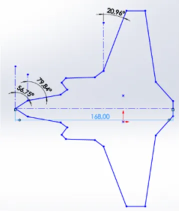
The F35 aircraft configuration is given in Fig. 1. The full-scale configuration has a thickness of 5 mm, mean aerodynamic chord length of 168 mm, bevel angle of 45°, and wing sweepback angle of the main wing is Λ = 20.96° and lower surface area of 137 cm2. The full-scale
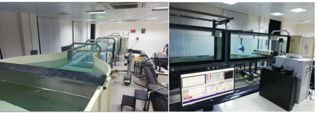
model was tested in a closed-circuit water channel experiment at the Department of Mechanical Engineering at Osmaniye Korkut Ata University. The closed-loop, open water channel experiment setup is given in Fig. 2. The experimental system consists of a water channel with dimensions of 750´1000´8000 mm (height ´ width ´ length) between two water tanks.
Figure 1: F35 aircraft configuration
Total water depth is 52 cm in the channel, water level under the wing is 20 cm and over the wing is 16 cm. The wall of the channel made from 15 mm thick transparent Plexiglas. The test was performed at a free stream velocity of 0.6 cm/s which corresponds to chord-based Reynolds number of 10.000. To provide uniform flow, there is a current regulator before the contraction section. Before the test section, water was directed into a settling chamber and passed through a honeycomb section where there is a channel contraction with the ratio 2:1. These two arrangements were used to preserve the turbulence intensity below 0.1%. Rhodamine 6G was used in the dye experiment, which shines under 532 nm laser light and was recorded using a SONY HD-SR1camera. The dye was injected at the apex from a certain height with a plastic pipe. There is a needle at the end of this pipe, which is placed in a channel along the central axis in the model aircraft. In the present dye experiment, the plan and side view flow pattern of the model was captured and presented at the angle of attack from 5° to 25°.
Figure 2: The closed-loop, open water channel experiment setup
Stereoscopic Particle Image Velocimetry (stereo-PIV) technique provides information about the instantaneous or time average values of flow structure by measuring the velocities of small metal-coated solid particles at the micron size, which is moving at the same speed as the fluid in the flow. In this experiment, 10-micrometer silver-coated plastic particles were added into water. Although the densities of the particles (1100 kg/m3) are relatively higher than the density
of the water, they move almost at the same speed as the water due to their micron size. A double pulsed 120 mJ power unit was used to produce a laser beam and converted into 1 to 2 mm thickness laser beam using an optical instrument. The time interval between consecutive pulses was set to 1.5 ms for all measurements. The pulsed laser unit can send up to 15 laser beam pairs per second. The consecutive motion of particles was recorded with a CCD camera with a resolution of 1600 ´ 1186 pixels. The camera-equipped lens with 60 mm focal length and 900 consecutive images were taken for each continuous run with an acquisition frequency of 15 Hz. Detail information about parameters, experimental, and PIV systems are available at the Ref. [16-20].
3.Numerical Approach
The flow field over the X45 wing was simulated by using commercial software COMSOL. Reynolds-Averaged Navier-Stokes (RANS) equation was applied for the conservation of momentum and the continuity. Turbulence effects were modeled by using the Menter Shear-Stress transport (SST) model with realizability constraints. The SST model is also called the low-Reynolds number model and this model resolves the flow field all the way down to the wall. SST model is expressed in terms of k and ω with Eqn. (1) and Eqn. (2) [21-23].
𝜌!" !#+ 𝜌𝑢. ∇𝑘 = 𝑃 − 𝜌𝛽$ ∗𝑘𝜔 + ∇. ((𝜇 + 𝜎 "𝜇&)∇") (1) 𝜌!' !# + 𝜌𝑢. ∇𝜔 = () *!𝑃 − 𝜌𝛽𝜔 ++ ∇. 0(𝜇 + 𝜎 '𝜇&)∇'1 + 2(1 − 𝑓,-) (."# ' ∇𝜔. ∇𝑘 (2)
where, P is the static pressure and can be represented with the Eqn. (3).
𝑃 = min (𝑃", 10𝜌𝛽$∗𝑘𝜔) (3)
Here, 𝑃" production term and it is expressed with Eqn. (4).
𝑃" = 𝜇&;∇𝑢: (∇𝑢 + (∆𝑢)&) −+/(∇. 𝑢)+> −+/𝜌𝑘∇. 𝑢 (4)
Turbulence viscosity is expressed with Eqn. (5), 𝜇& = (0$"
123 (0$',78%#) (5)
where, S is the characteristic magnitude of the mean velocity gradients and is expressed with the help of Eqn. (6).
𝑆 = @2𝑆:;𝑆:; (6)
The interpolation functions 𝑓,- and 𝑓,+ are represented with the Eqn. (7) and Eqn. (8).
𝑓,-= tanh D𝑚𝑖𝑛 H𝑚𝑎𝑥 ;=√" &∗'>", ?$$* ('>"#> , @(."#" 123 (#()"#" ∇'.∇",-$*$&)>"#K @ L (7) 𝑓,+= 𝑡𝑎𝑛ℎ O𝑚𝑎𝑥 ; √" =&∗'>", ?$$* ('>"#> + P (8) where, 𝑙' is the distance to the closest wall. For SST, default model constants are given by,
𝛽-= 0.075, 𝛾-=5
9, 𝜎"-= 0.85, 𝜎'-= 0.5, 𝛽+= 0.0828, 𝛾+ = 0.44, 𝜎"+ = 1.0, 𝜎C+= 0.856, 𝛽$∗= 0.09, 𝜎-= 0.31
For this calculation flow type was set to incompressible and gravity effect provided in the
z-direction. The delta wing had a chord length of C = 168 mm with a wing sweepback angle of Λ = 21.59. Wind speed was set to 0.058 m/s. Reynold's number was taken as 10,000 and flow over the boundary conditions of the wing was assumed to be turbulent. In a low Reynolds number model, the equations are integrated through the boundary layer to the wall, this allows a no-slip condition to be applied to the wing surface, therefore X45 wing was modeled as a solid wall with no-slip conditions and other boundaries was modeled as a free stream. The algebraic multigrid (AMG) solver with the generalized minimal residual (GMRES) method (a commercial version built-in COMSOL) was chosen because it is an iterative method for solving very large systems of
linear equations and provides robust solutions for large CFD simulations [24]. In the fluid flow problem, there are millions of equations or unknowns, proportional to the number of nodes in the finite element mesh therefore it is so expensive to solve with the direct solver. On the other hand, the iterative solver uses much less memory. Reynolds-Averaged Navier-Stokes (RANS) equation is solved in terms of averaged velocity and pressure fields in time. The turbulence effect is computed with two equations SST turbulence model. On the surface of the model aircraft, free triangular mesh type was applied and the minimum element size was limited as 0.0001 and maximum was set to 0.0005 then a total 177.766 triangular mesh element was generated. For the 3D computational domain, the tetrahedral mesh type was chosen and the minimum element size was limited to 0.0001 and maximum growth rate set to 1.25 and finally, 6 million tetrahedral mesh elements were generated. Low numbers of mesh lead to a calculation error, while too much mesh increases the calculation time considerably. If only the mesh number is in a certain range, the results are more agreement with the experimental data. For the numerical calculation in the literature, only criteria are generally compliant with the experiment. Therefore, the effect of the mesh number on the numerical results was carefully tested in preliminary calculations and the mesh configuration more agreement with the experiment was set. COMSOL has an integrated mesh generation and quality control module and mesh quality are generally checked in terms of skewness of the mesh element. In this study, mesh quality was checked and the average element quality was calculated 0.65, and minimum was 0.19. Mesh quality 1 is the best possible and it indicates an optimal element in the chosen quality measure and 0 is the worst. In general, elements with a quality below 0.1 are considered as poor quality for many applications [25]. Mesh distribution is given in Fig. 3. The simulation was carried out for the full model aircraft. To eliminate domain size effect on the calculation results, the computational domain size was extended at least over 10 times the chord length of the model. The upstream boundary was placed 20 mean aerodynamic chords in front of the apex, 20 mean aerodynamic chords behind the tail, and 10 mean aerodynamic chords above and below the pressure and suction side. This configuration is consistent with other numerical studies [26]. The inlet port was set to velocity inlet and outlet port was set to pressure outlet with zero atmospheric pressure and no-slip boundary condition was applied for the surface of the model. The computation was carried out with a server with 32 processors and 64 GB RAM. Detailed information about numerical method and equations are available at the Ref. [27, 28]
Figure 3: Mesh distribution around model aircraft
4. Results and Discussion
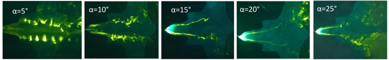
Dye visualization of the flow field structure of the model aircraft for the thickness of 5 mm in the plan view is presented in Fig. 4 at the angle of attack from 5° to 25°. At the lower angle of attack at α = 5°, flow is almost conventional and moves very orderly until at the end of the trailing edge side of the wing. However, at α = 10° small scale leading-edge vortex (LEV) develops and rotation of flow is evident at the lower side of the front body. Turbulence intensity increases compare to the previous image and there is cross current on the wing surface with lateral mixing. When the angle of attack increased to α = 15°, LEV and vortex breakdown are quite prominent on the main wing. By the time α = 20° is reached, flow is swirling from beginning to end and spiral vortex breakdown happens under the main wing surface. When the angle of attack increased to α = 25°, the size of rotation and turbulence increases and the location of the vortex breakdown moves forward. Although LEV keeps up its flow regime on the front side, it became quite unstable, and ruptures in flow become more common.
Figure 4: Dye visualization of the plan view with the formation and development of LEV and vortex breakdown
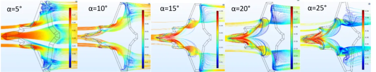
Fig. 5 shows the lower surface computational flow field with the formation and development of LEV and vortex breakdown. At the lower angle of attack such as α = 5°, streamline flowing under the surface of the model aircraft without lateral mixing and fluid flows in parallel layers until at the end of trailing edge side of wing or tail but behind the aircraft, small scale cross-currents or lateral mixing happens. When the increasing angle of attack up to α = 10°, a part of the flow field keeps flow regime the same but small-scale vortex develops along the leading-edge side of the body. The size of rotation is small and the cycle frequency is low. By the time α = 15° is reached, LEV is quite prominent, cycle frequency decreases, the radius of core
increases and vortex breakdown is happening on the wing surface. At this angle, the LEV gets under the influence of a larger and stronger vortex, which is the precursor of the vortex breakdown. At α = 20°, the vortex with a lower loop frequency appears to increase the effectiveness and disrupt normal LEV formation where circulating frequency decreases, size of LEV increases, and location of vortex breakdown moves to further up to the front side of the model. When the angle of attack increased to α = 25°, irregularities in the flow structure and size of vorticity increases at the rear side of the model, and the location of the vortex breakdown moves a little bit further to the front side. When the experimental and theoretical results are compared, there is a good correlation between the experiment and the numerical approach at the angle of attack from 5° to 25°.
Figure 5: Computational visualization of the plan view with the streamline velocity field with the formation and development of LEV and vortex breakdown
Fig. 6 shows PIV time-averaged vorticity field at the angle of attack from 5° to 25°. In the vorticity image, solid dark lines represent clockwise rotation, while dotted lines express a counterclockwise loop. At α = 5°, streamlines move in parallel layers and no disruption between the streamlines but vorticity image indicates two small scale formation of vortex area under the wing surface where one of them is on the body and the other is on the wing. The figures show the symmetric vortex area on both sides of the body and the wing surface. Both vorticity images represent LEV formation, but since the body does not consist of a single geometry like a simple delta wing, one represents LEV formation on the front while the other represents LEV formation on the wing. The same situation is seen also in Fig. 5 where fluids from different regions create both LEV separately and join at the back. As is seen in Fig. 6 (α = 5°) LEV develops along from front to the back across the entire wing surface and there is no situation to imply vortex breakdown but by the time α = 10° is reached, it appears that LEV flow regime ends at the backside of the wing where an irregular vortex area is formed and this proves the location and formation of vortex breakdown on the wing. When the angle of attack increased to α = 15°, LEV intensity decreases and the area it covers narrows, and LEV regime appears to be structurally impaired along the LEV axis. As the increasing angle of attack up to α = 20° flow regimes of the LEV shortens further and the point where the LEV ends is the beginning of the vortex breakdown. Finally, by the time α =
α=10° α=15° α=20° α=25°
25° is reached, LEV regime disrupts, location of the vortex breakdown moves forward and expands, and undesirable other vortex areas form in different places.
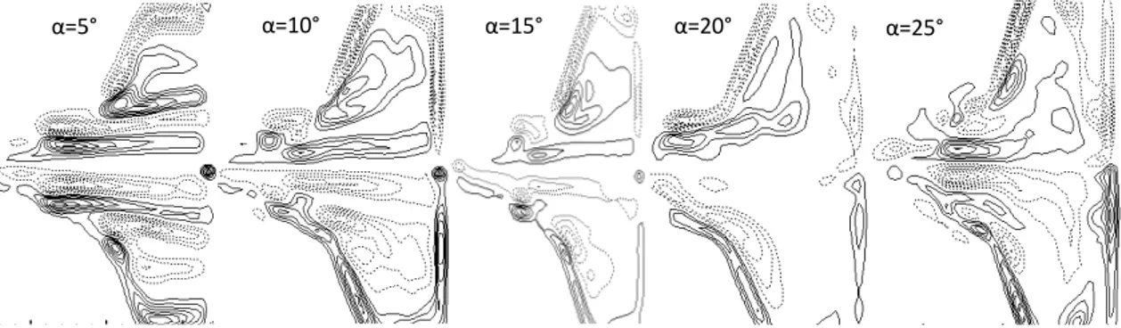
Figure 6: Patterns of the time-averaged vorticity, <ω> field of the model aircraft with the angle of attack
The plan view vorticity contour on the surface as a function of the angle of attack is given in Fig. 7. At α = 5°, The LEV regime extends from front to toe appears symmetrically on both sides of the body. Two LEV regimes are seen also in other previous figures. The first one is on the front, thinner and shorter, while the other is longer and wider, it covers the majority of the body from front to back. The LEV at the front extends along the outer line, while the LEV at the rear extends along the starting line of the wing on the body. Besides, there is a weaker third LEV regime on the wing closer to the tip. It was also observed in PIV experiments where three LEV regimes were formed and are seen in Fig. 6 (α = 15°). The main reason for the formation of different LEV flow regime is caused by the fact that the plane is not composed of a uniform geometry. By the time, α = 10° is reached, LEV regime in the front and on the body narrows, however third LEV, consist of two parts, in the middle outer part of the wing has expanded and strengthened. Apart from these three LEV flow regimes, it is seen that the fourth but irregular eddy currents begin to form on the backside of the wing. These irregular currents are the precursors of the vortex breakdown. When the angle of attack increased to α = 15°, the LEV regime on the middle body almost disappears, and the vortex area on the wings bends towards the edge and the second part of the third vortex becomes stronger. Irregular flows at the backside become stronger and merge to form vortex breakdown, and now covers at the middle backside of the wing. As the increasing angle of attack up to α = 20°, LEV transforms into a different vortex area on the wingtip, LEV regime retains its dominance in the front, and almost disappears in the middle part. The size of the vortex breakdown increases and location moves further up to the front side. Finally, by the time α = 25° is reached, LEV regime almost disperses, and the location of the vortex breakdown moves further but there is still LEV regime in the front side, and the size of the core increases close to wingtip.
Figure 7: Comparison of pattern of vorticity contour on the surface as a function of angle of attack
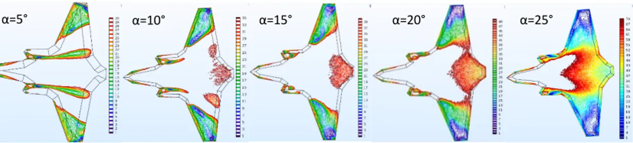
PIV streamline data of the F35 aircraft model is given in Fig. 8. At the angle of attack 5°, the flow regime is quite linear, and there is almost no turbulence happens on the surface. When the angle of attack increased to 10°, streamlines converge along the outer front lines of the model and indicates the formation of LEV. As the angle of attack increases, the flow lines get closer and tighter and show a circular behavior along the outer line of the wing. By the time α = 20° is reached, the figure indicates a vortex area on the outer side of the wing, which was also reported in Fig. 6 (α = 20°). Finally, by the time α = 25° is reached, the severity of the vorticity on the wing surface increases, and a circular core forms in the upper part.
Figure 8: Comparison of near-surface patterns of streamline topology of PIV experiment
5. Conclusions
A computational and experimental study was conducted for the F35 fighter jet configuration. In the experiment dye visualization and particle image velocimetry (PIV) techniques were used and plan view velocity field and vorticity pattern were presented. For the numerical part, Reynolds Average Navier Stokes (RANS) theorem equations with SST turbulence model were solved for incompressible flow around the wing surface and, were compared with experimental data to validate simulation accuracy of computational fluid dynamic approaches. In the dye visualization experiment, LEV development started at α = 10° vortex breakdown pronounced at 15°. When the increasing angle of attack, the location of the vortex breakdown moved further to the front side with increasing size and severity but never reached the apex. In the numerical study, vortex breakdown was observed firstly at the angle of 15°. As the increasing angle of attack, the size of the core increased with decreasing frequency. At 25°, there was still LEV regime in the front even it was small and there was no complete stall. In PIV experiment,
α=5° α=10° α=15° α=20° α=25°
LEV development started at α = 5°, three different LEV regimes were observed on the model. With the increasing angle of attack to 10°, a vortex area, transverse to the back of the plane was observed, which indicated the formation of a vortex breakdown. As the increasing angle of attack, LEV distance shortened and dispersed structurally, location of vortex breakdown moved to the front side but there was no complete stall condition observed. In the pattern of vorticity contour of numerical data, LEV pattern developed at the angle of attack at 5°, vortex breakdown showed signs of formation at 10° and became evident at 15° on the backside. With the increasing angle of attack, the area of irregular vortex formation (vortex breakdown) expanded and moved forward. In PIV experiment, streamline topology of the model was plotted and a steady flow was observed at 5°. As the increasing angle of attack, flow lines were gathered along the contours of the model and showed LEV formation. At 25°, the rotation core appeared to occur near the tip of the wings.
When the numerical results are compared with the experimental observations, there is a good agreement between them. The installation and operating costs of the experimental systems are quite high therefore, in the modern design process, the computational fluid dynamics method becomes an important analysis method together with the experiment. Experimental systems have the advantage of dealing with "real" fluid and can produce a much wider range of global data than CFD, but the experiment does not produce data in a wide range of Reynolds numbers. For example, it is subject to an important wall and boundary system fixes and is not very suitable for providing flow details. In modern aircraft design, it is necessary to focus on CFD with experimental systems. Nomenclature 𝑐D Pressure coefficient 𝑐E Lift coefficient 𝑓C- Damping fuction 𝑃 Static pressure 𝑃F Free stream pressure 𝑈G Relative velocity
𝑈F Free stream velocity (wind velocity) 𝑣 Kinematic viscosity
𝑐 Airfoil chord
𝑡 Percentage of the maximum thickness 𝑘 Turbulence kinetic energy
κ Von K𝑎́rm𝑎́n constant, 𝑙GH8 Reference length scale L Length scale of flow 𝜀 Turbulence dissipation rate 𝜔 Specific dissipation rate 𝜔# wall vorticity at the trip
𝜌F Freestream density 𝜇 Dynamic viscosity
S magnitude of the vorticity, 𝑆_ Modified vorticity
𝑆:; Mean strain rate
Ω:; Mean rotation rate
𝜇H88 Effective dynamic viscosity 𝛼 Angle of attack
∅ Scalar quantity of the flow CFD Computational Fluid Dynamics
NACA National Advisory Committee for Aeronautics NASA National Aeronautics and Space Administration
Acknowledgement
The authors wish to thank Osmaniye Korkut Ata University and Middle East Technical University providing technical support. This work was also supported by Adıyaman University Scientific Research Project (Project no: TEBMYOMAP/2018-0001).
References
[1] Waldmann, A., Unsteady wake flow analysis of an aircraft under low-speed stall
conditions using DES and PIV, In 53rd AIAA Aerospace Sciences Meeting, 1096, 2015.
[2] Yokokawa, Y., Murayama, M., Ito, T., Yamamoto, K., Experiment and CFD of a
high-lift configuration civil transport aircraft model, In 25th AIAA aerodynamic measurement
technology and ground testing conference, 3452, 2006.
[3] Johnson, F.T., Tinoco, E.N., Yu, N.J., Thirty years of development and application of
CFD at Boeing Commercial Airplanes, Seattle, Computers & Fluids, 34(10), 1115-1151, 2005.
[4] Sogukpinar, H., Numerical investigation of influence of diverse winglet configuration
on induced drag, Iranian Journal of Science and Technology, Transactions of Mechanical
Engineering, 44, 1-13, 2019.
[5] Gursul, I., Gordnier, R., Visbal, M., Unsteady aerodynamics of nonslender delta wings, Progress in Aerospace Sciences, 41(7), 515-557, 2005.
[6] Canpolat, C., Yayla, S., Sahin, B., Akilli, H., Dye visualization of the flow structure
over a yawed nonslender delta wing, Journal of Aircraft, 46(5), 1818-1822, 2009.
[7] Muir, R.E., Arredondo-Galeana, A., Viola, I.M., The leading-edge vortex of swift
wing-shaped delta wings, Royal Society Open Science, 4(8), 170077, 2017.
[8] Jardin, T., David, L., Spanwise gradients in flow speed help stabilize leading-edge
vortices on revolving wings, Physical Review E, 90(1), 013011, 2014.
[9] Yaniktepe, B., Rockwell, D., Flow structure on diamond and lambda planforms:
Trailing-edge region, AIAA journal, 43(7), 1490-1500, 2005.
[10] Yaniktepe, B., Ozalp, C., Canpolat, C., Aerodynamics and flow characteristics of
X-45 delta wing planform, Kahramanmaras Sutcu Imam University Journal of Engineering
[11] Canpolat, C., Yayla S., Sahin, B., Akilli, H., Observation of the Vortical Flow over a
Yawed Delta Wing, Journal of Aerospace Engineering, 25, 613-626, 2012.
[12] Watanabe, S., Kato, H., Stereo PIV applications to large-scale low-speed wind
tunnels, In 41st Aerospace Sciences Meeting and Exhibit, 919, 2003.
[13] Watanabe, S., Mungal, M.G., Velocity field measurements of mixing-enhanced
compressible shear layers, AIAA, 99-0088, 1999.
[14] Humphreys, W.M., A survey of particle image velocimetry applications in Langley
Aerospace Facilities, AIAA Paper, 93-0411, 1993.
[15] Wiegand, C., F-35 Air vehicle technology overview, 2018 Aviation Technology, Integration, and Operations Conference, 1-28, 2018.
[16] Raffel, M., Willert, C.E., Wereley, S.T., Kompenhans, J., Particle image velocimetry:
A practical guide, 2nd ed., Springer, 2007.
[17] Arroyo, M.P., Greated, C.A., Stereoscopic particle image velocimetry, Measurement Science & Technology, 2(12), 1181-1186, 1991.
[18] Westerweel, J., Digital particle image velocimetry, Theory and Application, Delft University Press, 1993.
[19] Adrian, R.J., Twenty years of particle image velocimetry, Experimental Fluids, 39, 159–169, 2005.
[20] Raffel, M., Willert, C.E., Wereley, S.T., Kompenhans, J., Particle image velocimetry:
A practical guide, 2nd ed., Springer, 2007.
[21] Menter, F.R., Two-equation Eddy-viscosity turbulence models for engineering
applications, AIAA Journal, 32(8), 1598-1605, 1994.
[22] Menter, F.R., Kuntz, M., Langtry, R., Ten years of ındustrial experience with the SST
turbulence model, Turbulence Heat and Mass Transfer, 4, 625-632, 2003.
[23] COMSOL CFD Module user guide, http://www.comsol.com (Accessed on April 8, 2019).
[24] Fontes, E., Using the algebraic multigrid (AMG) method for large CFD simulations, https://www.comsol.com (Accessed on April 8, 2019).
[25] Sogukpinar, H., Effect of hairy surface on heat production and thermal insulation on
the building, Environmental Progress & Sustainable Energy, e13435, 1-8, 2020.
[26] Cummings, R.M., Scott, A.M., and Stefan, G.S., Numerical prediction and wind
tunnel experiment for a pitching unmanned combat air vehicle, Aerospace Science and
Technology, 12(5), 355-364, 2008.
[27] Sogukpinar, H., Low speed numerical aerodynamic analysis of new designed 3D
transport aircraft, International Journal of Engineering Technologies, 4(4), 153-160, 2019.
[28] Sogukpinar, H., Numerical calculation of wind tip vortex formation for different