Central bank independence, government political orientation and optimum government expenditure financing

Central Bank Independence, Government Political Orientation and Optimum

Government Expenditure Financing

Article · December 2000 CITATIONS 0 READS 72 2 authors:

Some of the authors of this publication are also working on these related projects: Economic Performance and UnemploymentView project

Macroeconomic Plicy and UnemploymentView project M. Hakan Berument Bilkent University 145PUBLICATIONS   1,895CITATIONS    SEE PROFILE A. Özlem Önder Ege University 29PUBLICATIONS   244CITATIONS    SEE PROFILE

All content following this page was uploaded by M. Hakan Berument on 21 May 2014. The user has requested enhancement of the downloaded file.

Orientation and Optimum Government Expenditure

Financing

This paper extends the government optimum expenditure financing model by incorporating the effects of both the government’s political orientation and the central bank’s independence. For the panel data of fourteen OECD countries for the period from 1974 to 1997, this paper shows first that countries with higher levels of central bank independence generate less seigniorage revenue, and second that governments which are controlled by left-wing parties create more seigniorage revenue to finance their spending.

JEL Code: E61, E58 & E63

Key Words: Government Optimum Expenditure Financing Model, Central Bank Independence and Partisan Theory.

Central Bank Independence, Government Political

Orientation and Optimum Government Expenditure

Financing

Abstract

This paper extends the government optimum expenditure financing model by incorporating the effects of both the government’s political orientation and the central bank’s independence. For the panel data of fourteen OECD countries for the period from 1974 to 1997, this paper shows first that countries with higher levels of central bank independence generate less seigniorage revenue, and second that governments which are controlled by left-wing parties create more seigniorage revenue to finance their spending.

JEL Code: E61, E58 & E63

Key Words: Government Optimum Expenditure Financing Model, Central Bank Independence and Partisan Theory.

1. Introduction

This paper incorporates the effects of a government’s political orientation and the central bank’s independence into Mankiw’s (1987) government optimum expenditure financing model. For the panel data of fourteen OECD countries from 1974 to 1997, the paper finds that the choice between taxation and seigniorage to finance government spending is influenced by two additional factors: central bank independence (hereafter CBI) and the political orientation of governments (right-or left-wing governments). Empirical evidence suggests that seigni(right-orage revenue creation is lower for those countries that have more independent central banks or whose governments are right-wing. Alesina (1988, 1989), Grilli and Tabellini (1991), Cukierman, Webb and Neyapti (1992) and Berument (1998) find that countries with more independent central banks are associated with lower levels of inflation. Alesina & Sachs (1988), Chappell & Keech (1988) and Berument (1994) find that right-wing governments are associated with lower levels of inflation (or money creation) than left-wing governments. This study considers these two factors and tests whether they successfully explain governmental monetary policy determination within the governments’ optimum financing model.

A government’s monetary policy might be set along with its tax policies to generate revenue in order to finance spending. Mankiw argues that since both of these resources create inefficiencies in an economy, governments make use of these revenues together to finance spending. Mankiw (1987) and Poterba & Rotemberg (1990) find a positive relationship between tax and seigniorage revenues for the U.S. after World War II. However, Poterba & Rotemberg (1990) could not find the same positive relationship between a proxy of seigniorage revenue and tax revenue for France,

Germany and the U.K. They note that changing a government’s objective function and institutional factors may affect the tax-seigniorage trade off. This paper considers the government’s changing orientation and different degrees of central bank independence as additional factors and explores whether the relationship between tax and seigniorage revenue is influenced by these two factors.

When governments set up their monetary policies, they might also have other concerns, such as achieving higher growth levels or influencing interest rates. Considering the first of these other motives, Fischer (1977), Barro (1977 and 1978) and Barro & Gordon (1983) argue that govern-ments may use their monetary policies to influence the output and (/or) the unemployment rate. Regarding the second concern, Cukierman (1990) argues that central banks (hereafter CBs) have incentive to decrease interest rates by increasing money supply in order to secure the stability of the financial systems. This paper also considers these two alternative motives in the discussion of the empirical evidence for the implications of the optimum expenditure financing model. Taking these two motives into account does not, however, change the basic conclusion of the paper.

The models on the optimum financing literature use inflation as a proxy for government seignior-age revenue (e.g., Mankiw, 1987, Grilli, 1989, Poterba & Rotemberg, 1990, and Trehan & Walsh, 1990). However, seigniorage revenue is not the only factor that affects the inflation rate. As done in Berument (1994 and 1998), section 2 derives the implications of the optimum financing model when a government’s policy variables are the tax rate and the monetary base growth rate, not the tax rate and the inflation rate as some of the existing literature on the optimum financing model assumes. Furthermore, the effects of the orientation of the government and the CBI are

incorporated.1 Section 3 introduces the data, Section 4 covers the empirical evidence, and the last

2. The Theoretical Model

It is assumed that the monetary and fiscal branches of the government determine the govern-ment’s monetary and tax policies simultaneously. Tax and seigniorage revenue are ultimately used to finance government spending. Both the fiscal and the monetary branches like to minimize the present value of the burden of these two revenues. However, the monetary authority (the central bank) is more concerned with the loss generated by the seigniorage revenue than the fiscal

author-ity is.2 Therefore, we assume that generating the same amount of seigniorage revenue will be more

difficult if a CB is more independent. Hence, we can write the government’s objective function as

W_t= ∞ X s=0 (1 + r)−s " θ1+α_t+s − κ(cbi) µ_M t+s−1 M_t+s ¶_1−β# (1)

where W_t is the present value of the loss generated by taxation and seigniorage revenue, θ_t is the

tax rate and M_t is the monetary base (hereafter money) at time t, r is the fixed real interest rate,

cbi is the CBI index and κ(cbi) is the relative weight government assigns to seigniorage revenue

creation at any given level of taxation in the objective function. Here, θ_t1+α measures the loss

created by taxation and −

³

Mt−1

Mt

´_1−β

measures the loss generated by the seigniorage revenue at time t. Moreover, α and β are non-negative constants, and hence, the deadweight loss function for

each type of government, W_t, is a convex function of both the tax rate and money growth in order

to satisfy the second order conditions. It is assumed that κ(cbi) is an increasing function of CBI3,

so it will be more difficult for the government to increase the money growth in countries which are associated with more independent CBs, ceteris paribus.

It is important to note that we also allow that different types of administrations (type D and type R) assign different weights to the creation of seigniorage revenue for a given level of taxation

can be written as W_ti= ∞ X s=0 (1 + r)−s " θ1+α_t+s − κi(cbi) µ_M t+s−1 M_t+s ¶_1−β# i =D,R. (2)

As in the similar model of Alesina and Sachs (1988), it is assumed that Party R is more sensitive to

money growth than Party D; hence, κR(cbi) is greater than κD(cbi) at the given level of CBI, cbi.

Therefore, the objective function as stated in equation 2 allows that any type of administration derives loss from both the seigniorage revenue and taxes. The seigniorage loss is higher for a given level of taxation if the government is type R rather than type D, and if the central bank is more independent.

Here, we assume that the CB is sensitive to the creation of seigniorage revenue for both types of administrations at different degrees for each level of the central bank independence index. In other words, under complete central bank independence, the orientation of government affects the seigniorage revenue creation differently. There are two reasons for this: first, Cukierman(1992) recognizes that there is no completely independent central bank that is insensitive to political

pressure from the government. Second, allowing the possibility that κD(cbi) and κD(cbi) converge

under complete central bank independence requires imposing some arbitrary non-linear functional forms of κ(.). The results of this paper could be sensitive to functional form selection.

The intertemporal budget constraint the government faces when it chooses to minimize its loss function requires that the government debt be equal to the debt and its interest payments from the previous period plus government spending minus government tax and seigniorage revenues. Here, the seigniorage revenue is written as

M_t− Mt−1 P_t = µ 1−Mt−1 M_t ¶ m_t (3)

intertemporal budget constraint is written as b_t= (1 + r)b_t−1+ G_t− θ_ty_t− µ 1−Mt−1 M_t ¶ m_t (4)

where b_t is government debt, G_t is real government spending, and y_t is real income at time t.

Governments set the tax rate, θ_t and the inverse of the monetary base growth, M_Mt−1

t to minimize

their objective function, Equation 2, subject to their intertemporal budget constraint, Equation 4. The Hamiltonian equation can be written as

H =P∞_s=0(1 + r)−s · θ_t+s1+α− κi_(cbi)³Mt+s−1 Mt+s ´_1−β¸ − λ_t³rb_t−1+ G_t− θ_ty_t− ³ 1−M_Mt−1 t ´ m_t´ i =D,R. (5)

The first order conditions require that the marginal loss of taxation and seigniorage must be equal to each other. For both types of administrations the marginal loss of taxation is

(1 + α)θα

(1 + ε_θ)y_t (6)

Here, ε_θis the constant elasticity of real income with respect to the tax rate. Poterba and Rotemberg

suggest including ε_θ to incorporate the feedback effects of taxation into real income. The marginal

loss of money growth for each type of administration is equal to (1− β)κi(cbi)(M_t−1/M_t)−β

m_t(1− ε_µ) i =D,R. (7)

where the constant elasticity of real money holdings with respect to the change in money growth,

ε_µ, is also incorporated in order to account for the effect of money growth on real money holdings

because money growth, which causes inflation, affects the opportunity cost of holding money. It is important to note that higher CBI causes the marginal loss of the money growth rate to be higher for both parties. However. the marginal deadweight loss due to money growth is different for each party. For each type of administrations, the first order conditions will give the following after equating the logarithms of Equations 6 and 7 for each type of government:

ln Mt M_t−1 = 1 βln (1 + α)(1− ε_µ) (1− β)(1 + ε_θ) + α βlnθt+ 1 βln m_t y_t − 1 βlnκi(cbi) i =D,R. (8)

The equations are combined with a dummy variable D_t for both types of administration. D_t will have a value of one if the government is type D, and zero otherwise. Furthermore, it is assumed

that κi(cbi) = eδicbi, where δR is greater than δD, because it is assumed that type R governments

are more sensitive to money growth than type D governments. Hence, the following equation can be written ln Mt M_t−1 = 1 βln (1 + α)(1− ε_µ) (1− β)(1 + ε_θ) + α βlnθt+ 1 βln m_t y_t − 1 βδRcbi + 1 β(δRcbi − δDcbi)Dt (9)

Mankiw (1987) notes that government preferences towards tax and seigniorage creation might change over time and the cost of tax collecting is time variant. This paper investigates whether a substantial part of the seigniorage revenue creation can be explained by the optimum financing model under different institutional and political factors rather than by an exact relationship between tax and seigniorage revenue creation. Hence, to explain the behavior of seigniorage revenue under these two institutional factors, a simple error term is included. The following equation will be estimated. ln Mt M_t−1 = γ0+ γ1lnθt+ γ2ln m_t y_t + γ3cbi + γ4(Dt∗ cbi) + εt (10) Here, γ₀ = _β1ln(1+α)(1−ε_{(1−β)(1+ε}µ) θ), γ1 = α β, γ2 = 1β, γ3 = −δ R β , and γ4= −δ D_+δR

β . The testable implications

of the model are that γ₁, γ₂ and γ₄ are positive, and γ₃ is negative. The optimum financing model

suggests that there is a positive relationship between tax and seigniorage revenues. Equation 10 also suggests that less seigniorage revenue will be created if the CB is more independent. Moreover,

this specification, which includes the interactive term between D_tand cbi, allows us to test whether

the creation of the seigniorage revenue is lower for the type D administrations, compared to type

R administrations, for any given level of the central bank independence index. Note that both θ_t

and Mt

Mt−1 are in logarithmic terms. Hence, higher CBI not only causes the level of

Mt

but also causes a proportion of spending to be financed with less seigniorage revenue.

3. Data

The data set includes annual observations from fourteen developed OECD countries for the period from 1974 to 1997. Observations from developed countries, rather than from developing or less developed countries, are used because the optimum financing model implicitly assumes that governments can increase their tax revenues along with their seigniorage revenues if they wish to do so. On the other hand, developing countries may have difficulties in raising their tax revenues due to a less developed tax collection infrastructure. The data set includes observations from Australia, Austria, Canada, Denmark, Finland, France, Germany, Ireland, Italy, Japan, the Netherlands, Norway, the United Kingdom, and the United States.

Sources for data are as follows. The consumer price index (hereafter CPI), monetary base, GDP are from the International Monetary Fund-International Financial Statistics tape. Central

govern-ment spending and receipts5 are from OECD National Accounts, Income and Outlay Transactions

of General Government. The data for the type of regime is from Alesina (1989), and extended by Lane, McKay and Newton (1997).

The following are the descriptions of the variables that are used for the empirical test of the testable models. Money growth rate is the first logarithmic difference of the monetary base. The inflation rate is measured as the first logarithmic difference of the CPI. The logarithm of the tax rate is the logarithm of the central government’s receipt-GDP ratio. The first logarithmic difference of the monetary base is then used as a proxy for the seigniorage revenue. A direct way of measuring the seigniorage revenue is suggested by Klein & Neumann (1990). However, measuring the seigniorage revenue creation by using the method they suggest depends on legal, institutional and operational details of the monetary base creation, which cannot be compared across countries, as these two

authors mention. Because this study needs a proxy of seigniorage revenue that can be compared across countries, a new variable is not calculated but instead monetary base growth and inflation are used as a measure of seigniorage revenue.

Since it is very difficult to measure the CB’s actual independence, a central bank’s independence is measured as the legal independence of the central bank from its own government. Various central banks’ legal independence indexes have been calculated. The Cukierman, Webb and Neyapti (1992) (hereafter CWN) index is the most comprehensive and detailed one. Although we use the CWN index for the regression analysis, for completeness the next section reports the summary of the

estimates when the Bade & Parkin (1985) and Grilli et al. (1991) indexes are used.6

In their index, CWN consider sixteen different variables to construct the CB’s legal indepen-dence. They assign the variables values from zero to one, and then take the mean of those variables as the CB’s independence index. First, CWN consider policy formulation: who formulates mone-tary policy, how the CB carries out government directives, and how a conflict between the CB and government is resolved. The role that the CB plays in the formulation of the government budget is the final criterion examined in this category. Second, they study the appointment procedure for the bank. In this category, they consider the term of office, appointment and dismissal procedures, and the possibility of the governor holding a different office. Moreover, they incorporate the role of the price stability objective as stated in their charters to set up the CB’s independence index. Finally, they analyze the CB’s role regarding lending. Limitations on advances and saucerized lending, types of limits, the amount of control the CB has on terms of lending, and problems of lending in primary markets are some of the criteria considered in this category. Then the length of maturity of loans, restrictions on interest rates, and the extent of the CB’s circle of potential borrowers are analyzed to determine these factors’ contribution to the bank’s independence index. Appendix B also discusses other CBI indexes that are used later in the paper.

4. The Empirical Evidence

This section considers empirical evidence for two models. Equation 10 will be estimated in order to test the implication of the first model. The empirical evidence when the seigniorage revenue is proxied by the inflation rate will be also presented as a second model. The second model’s derivation appears in Appendix A.

To estimate these models, the Parks (1967) method is used. The method performs generalized least squares across countries and calculates the estimates by considering any autocorrelation for each country, for any variance difference across countries, and for any cross-country correlation. The method also constrains the estimated coefficients for each country such that each variable has the same estimated coefficient across countries. Constraining the estimated coefficients is necessary because the CBI index is prepared as a constant number for the entire period for each country. If the coefficients are not constrained, the estimates of the coefficients will not be obtained due to the perfect multicolliniarity problem.

Insert Table 1 about here

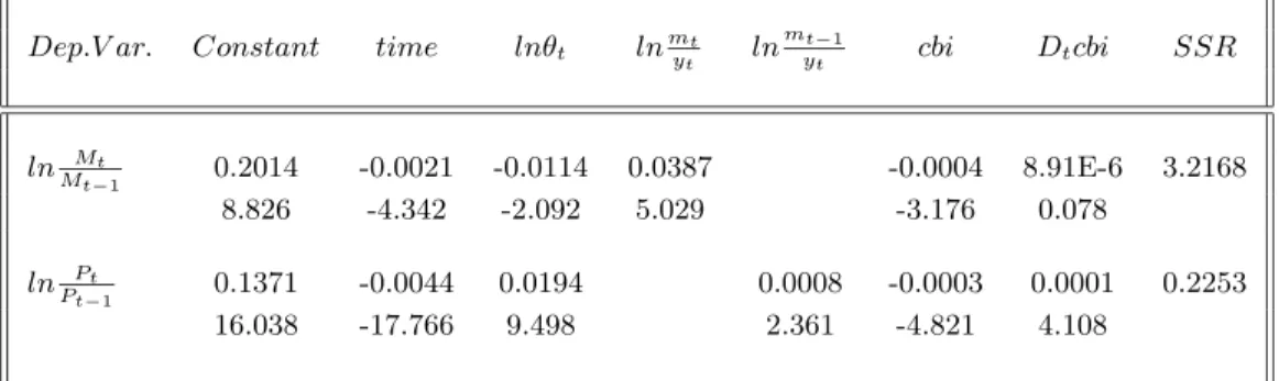
Table 1 reports the results for the two models. Before estimating the model, the time trend is

included in the regression analysis.7 Both the money growth rate (or inflation) and tax rates are

persistent variables. Performing a single regression analysis for Equation 10 may capture the time trend they share. The first row of the table is for the money growth rate-tax rate relationship (first model) suggested by Equation 10. Estimates for the inflation-tax rate relationship (second model) that Poterba and Rotemberg suggest are reported in the second row. The estimated coefficient for the logarithm of the tax rate is positive for inflation-tax rate relationship and negative for the money growth rate-tax rate relationship. This result suggests that there is a positive relationship between tax and seigniorage revenues that the optimum financing model suggests when inflation rate is used

as a proxy for seigniorage revenue and the coefficient for the model is statistically significant at

the 5% level.8 However, we could not find supporting evidence for the optimum financing model

for the money growth rate- tax rate relationship. The estimated coefficients for the CBI index are negative and significant; when countries have relatively more independent CBs, then they create less seigniorage revenue to finance their spending, ceteris paribus. As the theory suggests, the interactive dummies have a positive and statistically significant coefficient for the inflation-tax rate regression and a positive coefficient for money growth rate-tax rate regression. This suggests that the creation of the seigniorage revenue is lower for the type D administration, compared to type R administrations, at any given level of the central bank independence index. Hence, the creation of seigniorage revenue is not only lower for the countries associated with more independent central banks, but it is also higher if the administration is type D rather than type R. Lastly, coefficients on the logarithms of the money-income ratios are positive and significant as suggested by Equation 10. There is a feedback effect from the creation of seigniorage and tax revenues to real money holdings and the national output, respectively. The sums of squared residuals (SSRs) are also reported in the last column. In summary, only one implication of the optimum financing model – which suggests a positive relationship between money growth rate-tax rate – is rejected for the first specification. The implications of the hypotheses are all supported for the second model at least at the 5% level. One might consider the possibility that the positive relationship between seigniorage revenue and the tax rate is proxying a relationship other than that suggested by the optimum financing model. To test for this possibility, this study performs regression analyses after taking into account other possible influences. First, business cycles may influence government financing. Therefore, a proxy for business cycles is included in the regression analysis on an ad hoc basis to control for the business cycle effect. Second, CBs might be responding to the interest rate or the government deficit. Fiscal authority does not have complete control over the interest rate; changes in government deficit

or in government spending at a given level of taxes may also affect interest rates. Higher levels of government spending will increase the interest rate, and in order to decrease it the interest rate sensitive CB may increase the money supply. To incorporate this possibility, government spending is also included in the analysis. Hence, both the deviation of the real GDP from the trend expressed

as a ratio of trend-real GDP, υ_t, and the logarithm of the government spending-GDP ratio, lng_t,

are included in the regression analysis.

Insert Table 2 about here

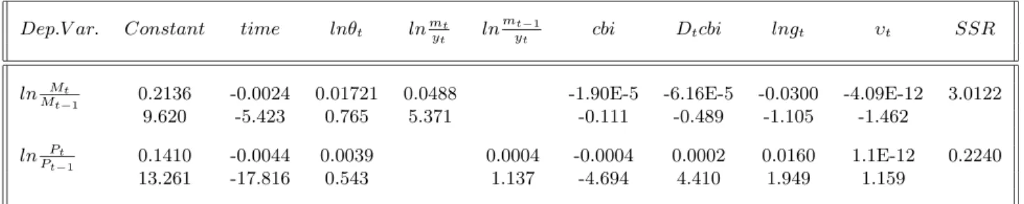
Table 2 reports the results after including two additional variables, υ_tand lng_t, in the models.

The results from Table 2 are weaker than the results from Table 1. For the money growth rate-tax rate relationship, the estimated coefficient for the tax rate becomes positive but insignificant and the coefficient for the central bank independence index is insignificant. The coefficient for the partisan effect is negative but insignificant. The second model is more robust relative to the first one. All of the coefficients have the same sign as those in Table 1. Furthermore, their level of significance is similar to their level in Table 1, except the coefficient for the tax rate and monetary base-GDP ratio, which are insignificant. Thus, the implications of the theory are not rejected for either of the models. The estimated coefficients for government spending do not support the implication of deficit financing or the interest rate smoothing hypothesis for the first model. The estimated

coefficient for lng_t is negative and insignificant for the money growth-tax rate relationship. On

the other hand, in the second model, the estimated coefficient lng_tis positive and significant. The

results appearing the literature are mixed as well. Evans (1988 and 1989) shows that government spending or deficit does not affect the interest rate for the U.S.. The estimated coefficients for the deviation of output from trend, however, are statistically insignificant for both the money growth rate-tax rate and the inflation-tax rate relationships. This may suggest that governments may not be persistently using their monetary policies to influence output level.

It is also necessary to consider that estimates reported in Tables 1 and 2 might be suffering from simultaneity biasedness. The theory presented in Section 2 assumes that governments determine their tax and seigniorage revenues simultaneously. Furthermore, the first order conditions also imply that the marginal deadweight loss of taxation (or money growth) must be the same across time. Hence, both the tax rate and the money growth rate are martingale and therefore, both are also endogenous variables, as is the logarithm of the money-income ratio because the tax rate and the money growth rate affect real income and real money holdings, respectively. Therefore, the instrumental variables (hereafter IV) are used to reestimate the models. The instruments are the lagged value of the logarithm of tax rate, the lagged value of the deviation of real GDP from the trend – expressed as a ratio of trend-real GDP, the lagged value of the logarithm of government spending-GDP ratio and a time trend. In order to perform the IV technique, the ordinary least squares method is used for both the first and second stage regressions.

Insert Table 3 about here

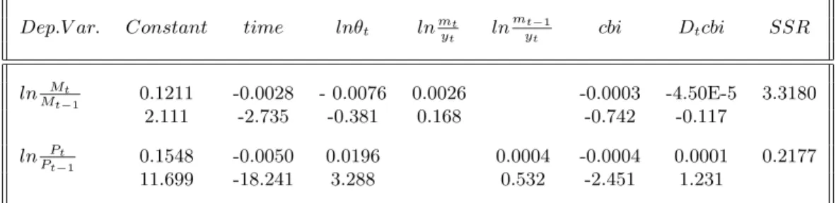
These results are reported in Table 3. The estimated coefficients for the money-income ratio are positive and those for the CBI indexes are negative, as the theory suggests, for both relationships. The interactive dummy is positive for the second model as the theory suggests. The coefficient of the tax rate is not significant for the money growth rate-tax rate relationship. The coefficients of the money-income ratio and the interactive dummy for government commitment are not significant for the inflation-tax rate relationship. Hence, the supporting evidence is diminished when the IV technique is used, although the implications of the theory are not rejected.

Insert Table 4 about here

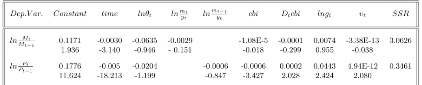
Table 4 reports the results when the IV technique is used to test the implications of the optimum financing hypothesis after considering the governments’ other possible motives. The estimates

reported in Table 2 did not change their signs for CBI and its interactive dummies for both of the models; however, none of the coefficients are significant for the money growth rate-tax rate relationship. The estimated coefficients for the tax rate and money-income ratio become negative for the inflation-tax rate relationship but they are not significant. Furthermore, the estimated

coefficient for the lng_tis positive and significant, just as in Table 2. However, the coefficient for υ_t

is positive and significant for the inflation-tax rate relationship.

A possible reason for the diminished supporting evidence when the IV technique is used is that there is a simultaneity bias problem for the regression analysis, which uses the Parks method. However, the reason might alternatively be that the IV method gives less efficient estimates than the Parks method.

It can be concluded that the estimated coefficients for the tax rates and interactive dummies are positive and the coefficients for the CBI are always negative, as the theory suggests for the inflation-tax rate relationship. The supporting evidence weakens under alternative hypotheses and also when the IV technique is used. This result is especially valid for the money growth rate- tax rate relationship.

4.1. Results when other indexes are used

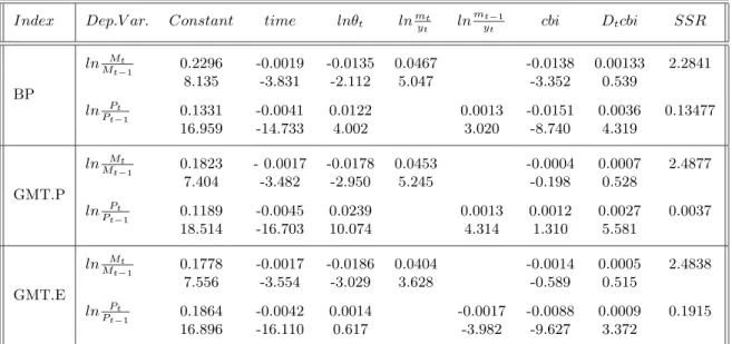
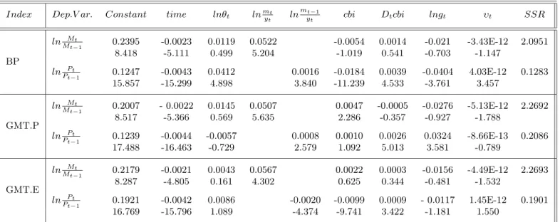
This subsection presents a summary of the evidence on the optimum financing model when three other indexes are used in addition to the CWN index for central bank independence. The estimated coefficients for the regression analysis, when all the indexes are used, are reported in Appendix C. An additional index has been taken from Bade & Parkin (1985) (hereafter BP), and the political and economic independence indexes are taken from Grilli et al. (1991) (hereafter GMT.P and GMT.E respectively.)

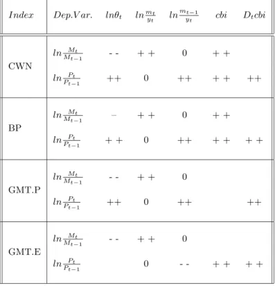
Table 5 reports the results for both the money growth rate- tax rate relationship and the inflation-tax rate relationship for all four CBI indexes. The BP index is not available for Austria, Finland and Ireland and the GMT.P and GMT.E indexes are not available for Finland and Norway; thus, these countries are excluded from the sample when the corresponding indexes are used. To save space, estimated coefficients for the constant term and the time trend are not reported. Furthermore, if an estimated coefficient has the sign the model suggests and is significant at the 5% (10%) level, then ++ (+) is reported. If the implication of the hypothesis is rejected at the 5% (10%) level, then – – (–) is reported for the corresponding variable. Lastly, 0 is reported when a variable is excluded from the regression.

Insert Table 6 about here

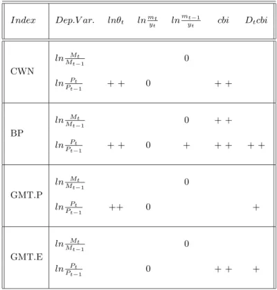
Table 5 shows that none of the implications of the hypotheses are rejected except the coefficient of the tax rate for the money growth rate-tax rate relationship and the coefficient of the indepen-dence index when GMT.E index is used for the inflation-tax rate relationship. When the CWN and the BP indexes are used, both types of relationships support the implications of the hypotheses more strongly than when the GMT.P and GMT.E indexes are used. Furthermore, the implications of the hypotheses are supported better by the inflation-tax rate relationship than by the money growth rate-tax rate relationship. Table 6 reports the same analysis when the IV technique is used. Even though none of the implications of the hypotheses are rejected, the supporting evidence

diminishes.9

Insert Table 7 about here

In sum, the hypotheses are mostly supported when the Parks estimation procedure is used, and the supporting evidence decreases when the IV technique is used. Lastly, when GMT.E’s and GMT.P’s independence indexes are used, the hypotheses are supported least. The most supporting

evidence is observed when the BP index is used.

5. Conclusion

The aim of this paper is to incorporate the effects of central bank independence and the political orientation of governments in the tax-seigniorage revenue trade-off, which governments face to finance their spending. The hypotheses tested in this paper are as follows: first, governments raise both their tax and seigniorage revenues together to finance spending; second, governments that are associated with more independent central banks create less seigniorage revenue; and third, the creation of seigniorage revenue is higher under left-wing governments at each given level of central bank independence.

The existing literature on the optimum financing uses inflation as a proxy for the government’s seigniorage revenue. The inflation rate might be affected by various factors other than the seignior-age revenue. The empirical results are found to be sensitive to different proxies of seigniorseignior-age revenue. When the seigniorage revenue is proxied by the monetary base growth rate, weaker sup-porting evidence is observed. The hypotheses of the paper are supported best when the CWN’s and the BP’s central bank independence indexes are used and when the seigniorage revenue is proxied by the inflation rate for fourteen OECD countries for the sample from 1974 to 1997. The supporting evidence decreases under alternative hypotheses and also when the IV technique is used.

These results are on a parallel with the relevant literature on CBI (e.g., Cukierman, 1992, Alesina and Summers, 1993, and Berument, 1998), which suggests that more CBI leads to less inflation. Moreover, the paper successfully demonstrates that the CBI and the political orientation of a government do influence the tax-seigniorage trade-off that governments face.

References

Alesina, A. (1988) Macroeconomics and politics, NBER Macroeconomic Annual 1988, (MIT Press, Cambridge, Mass).

Alesina, A. (1989) Politics and business cycles in industrial democracies, Economic Policy, April, pp. 55-98.

Alesina, A. & Sachs, J. (1988) Political parties and the business cycle in the United States, 1948-1984,

Journal of Money,Credit and Banking, 23, pp. 63-82.

Alesina, A. & Summers, L.H. (1993) Central bank independence and macroeconomic performance: Some comparative evidence, Journal of Money, Credit and Banking, 25, pp. 151-162.

Alesina, A. & Tabellini, G. (1987), Rules and discretion with noncoordinated monetary and fiscal policies, Economic Inquiry, 25, pp. 619-630.

Bade, R. & Parkin, M. (1985) Central bank law and monetary policy, manuscript.

Barro, R. J. (1977) Unanticipated money growth and unemployment in the US, American Economic

Review, 67, pp. 101-15.

Barro, R. J. (1978) Unanticipated money, output and price level in the US, Journal of Political

Economy, 86, pp. 549-80.

Barro, R.J. & Gordon, D. (1983) Rules, discretion and reputation in a model of monetary policy,

Journal of Monetary Economics, 12, pp. 101-122.

Berument, H. (1994) Political parties and optimum government financing, Southern Economic

Jour-nal, 61, pp. 510-518.

Berument, H. (1998) Central bank independence and financing government spending, Journal of

Macroeconomics, 20(1), pp. 133-151.

Burdekin, R. C.K. (1991) Inflation and taxation with optimizing governments: a comment, Journal

Chappell, H. W. & Keech, W. R.(1988) The unemployment rate consequences of Partisan monetary policies, Southern Economic Journal, 55, pp. 107-122.

Cukierman, A. (1990) Why does the Fed smooth interest rates? in: M. T. Belongia (Ed.), Monetary

Policy on the Fed’s 75th Anniversary. Proceedings of the 14th annual Economic Policy Conference

of the Federal Reserve Bank of St. Louis. Norwell, MA (Kluwer Academic Publishers).

Cukierman, A. (1992) Central Banks Strategy, Credibility, and Independence: Theory and Evidence, (MIT Press, Cambridge, Mass).

Cukierman, A., Webb, S. & Neyapti, B. (1992) The measurement of central bank independence and its effect on policy outcomes, The World Bank Economic Review, 6, pp. 353-398.

Evans, P. (1988) Are government bonds net wealth? Evidence for the United States, Economic

Inquiry, 26, pp. 551-566.

Evans, P. (1989) A test of steady state government-debt neutrality, Economic Inquiry, 27, pp. 39-55. Fischer, S. (1977) Long-term contracts, rational expectations, and the optimum money supply rule,

Journal of Political Economy, 85, pp. 191-205.

Grilli, V. (1989) Seigniorage in Europe, in : M. De Cecco & Gionannini A. (Eds.) A European Central

Bank?, (Cambridge University Press, Great Britain).

Grilli, V., Masciandaro, D. & Tabellini, G.(1991) Political and monetary institutions and public financial policies in the industrial countries, Economic Policy, 13, pp. 341-392.

Klein, M. & Neumann, M. (1990) Seigniorage: What is it and Who Gets it?,

Weltwirtschaftliches-Archiv, 126(2), pp. 205-21.

Lane, J., McKay, D. & Newton, K.(1997) Political Data Handbook OECD Countries, (Oxford Uni-versity Press, New York).

Mankiw, N. G. (1987) The optimal collection of seigniorage: Theory and evidence, Journal of

Parks, R.W. (1967) Efficient estimation of a system of regression equations when disturbances are both serially and contemporaneously correlated, Journal of American Statistical Association, 62, pp. 500-508.

Poterba, J. M. & Rotemberg, J. (1990) Inflation and taxation with optimizing governments, Journal

of Money, Credit, and Banking, 22, pp. 1-18.

Trehan, B. & Walsh, C. E.(1990) Seigniorage and tax smoothing in the United States, 1914-1986,

Notes

∗ We wish to thank Anita Akka¸s, Anwar El-Jawhari and Richard Froyen for their helpful

com-ments.

1. In Appendix A, the implication of the optimum financing model is derived when the govern-ment’s policy variables are the inflation and tax rates.

2. Both the monetary authority and the fiscal authority are subject to different political incentives and institutional constraints; therefore, they may differ on how to value the loss generated from tax and seigniorage revenues.

3. A similar approach is also used by Tabellini (1986) to incorporate CBI into governments’ objective functions.

4. Partisan theory assumes that parties represent their constituencies. It is reasonable to assume that these constituencies have fixed preferences for the tax rate and the money growth rate over the party’s time horizon. Therefore, it is considered (like in Alesina & Sachs, 1988, and Cukierman et

al. 1992) that once party D (or R) is elected, it will minimize its objective function for an infinite

horizon.

5. Government receipt figures for the US were obtained from the Department of Commerce, Bu-reau of Economic Research because the figures were not available from the International Monetary Fund-International Financial Statistics for the sample period this paper considers.

6. CBI indexes are calculated over different periods of time for several countries. These rankings are calculated as a constant number for the entire period that is considered for each country.

7. Mankiw and P&R also include the time trend in their models before testing. 8. The level of significance is 5% unless otherwise noted.

9. The regression analyses are also performed after controlling for the government’s possible other concerns. The results are parallel to the ones reported in Tables 5 and 6. All of the estimates for

Tables

Table 1: The Empirical Evidence on the Optimum Financing Model: 1974-1997.a

Dep.V ar. Constant time lnθt lnmt_yt lnm_ytt−1 cbi Dtcbi SSR

ln_Mt−1Mt 0.2014 -0.0021 -0.0114 0.0387 -0.0004 8.91E-6 3.2168

8.826 -4.342 -2.092 5.029 -3.176 0.078

ln_Pt−1Pt 0.1371 -0.0044 0.0194 0.0008 -0.0003 0.0001 0.2253

16.038 -17.766 9.498 2.361 -4.821 4.108

Note: lnθt = Logarithm of the tax rate; lnmt_yt = Logarithm of the real monetary base-real GDP ratio; lnm_ytt−1 = Logarithm of the lag value of the real monetary base-real GDP ratio; cbi = Central bank independence index; D_t= Dummy variable for the left-wing governments.

Table 2: Robustness Tests: 1974-1997.a

Dep.V ar. Constant time lnθ_t lnmt_yt lnmt−1_yt cbi D_tcbi lng_t υ_t SSR

ln_Mt−1Mt 0.2136 -0.0024 0.01721 0.0488 -1.90E-5 -6.16E-5 -0.0300 -4.09E-12 3.0122

9.620 -5.423 0.765 5.371 -0.111 -0.489 -1.105 -1.462

ln_PPt

t−1 0.1410 -0.0044 0.0039 0.0004 -0.0004 0.0002 0.0160 1.1E-12 0.2240

13.261 -17.816 0.543 1.137 -4.694 4.410 1.949 1.159

Note: lngt = Logarithm of government spending-GDP ratio; υt= Deviation of real GDP from trend expressed as a ratio of trend- real GDP.

Table 3: The Empirical Evidence on The Optimum Financing Model – IV Results: 1974-1997.a b

Dep.V ar. Constant time lnθ_t lnmt_yt lnmt−1_yt cbi D_tcbi SSR

ln_MMt

t−1 0.1211 -0.0028 - 0.0076 0.0026 -0.0003 -4.50E-5 3.3180

2.111 -2.735 -0.381 0.168 -0.742 -0.117

ln_Pt−1Pt 0.1548 -0.0050 0.0196 0.0004 -0.0004 0.0001 0.2177

11.699 -18.241 3.288 0.532 -2.451 1.231

a_{t-ratios are reported under the corresponding estimated coefficients.}

b _{Instruments are the lagged value of the logarithm of tax rate, the lagged value of the deviation of real GDP from} trend expressed as a ratio of trend-real GDP, the logarithm of the lagged government spending-GDP ratio, the time trend.

Table 4: Robustness Tests – IV Results: 1974-1997.a b

Dep.V ar. Constant time lnθt lnmt_yt lnmt−1_yt cbi Dtcbi lngt υt SSR

ln_Mt−1Mt 0.1171 -0.0030 -0.0635 -0.0029 -1.08E-5 -0.0001 0.0074 -3.38E-13 3.0626

1.936 -3.140 -0.946 - 0.151 -0.018 -0.299 0.955 -0.038

ln_PPt

t−1 0.1776 -0.005 -0.0204 -0.0006 -0.0006 0.0002 0.0443 4.94E-12 0.3461

11.624 -18.213 -1.199 -0.847 -3.427 2.028 2.424 2.080

a_{t-ratios are reported under the corresponding estimated coefficients.}

b _{Instruments are the lagged value of the logarithm of the tax rate, the lagged value of the deviation of real GDP} from trend expressed as a ratio of trend-real GDP, the logarithm of the lagged government spending-GDP ratio, the time trend.

Table 5: The Empirical Evidence on the Optimum Financing Model with Other Indexes: 1974-1997.

Index Dep.V ar. lnθt lnmt_yt lnmt−1_yt cbi Dtcbi

ln_Mt−1Mt - - + + 0 + + CWN ln_PPt t−1 ++ 0 ++ + + ++ ln_MMt t−1 – + + 0 + + BP ln_PPt t−1 + + 0 ++ + + + + ln_MMt t−1 - - + + 0 GMT.P ln_PPt t−1 ++ 0 ++ ++ ln_MMt t−1 - - + + 0 GMT.E ln_Pt−1Pt 0 - - + + + +

Table 6: The Empirical Evidence on the Optimum Financing Model with Other Indexes - IV Results: 1974-1997.

Index Dep.V ar. lnθ_t lnmt_yt lnmt−1_yt cbi D_tcbi

ln_Mt−1Mt 0 CWN ln_Pt−1Pt + + 0 + + ln_Mt−1Mt 0 + + BP ln_Pt−1Pt + + 0 + + + + + ln_Mt−1Mt 0 GMT.P ln_Pt−1Pt ++ 0 + ln_Mt−1Mt 0 GMT.E ln_Pt−1Pt 0 + + +

Table 7: Correlation Among Various Central Banks’ Independence Indexesa CWN BP GMT.P GMT.E CWN 1.000 0.67821 0.79581 0.56165 0.0 0.0153 0.0020 0.0574 BP 1.000 0.44281 0.45702 0.0 0.2000 0.1842 GMT.P 1.000 0.64897 0.0 0.0224 GMT.E 1.000 0.0 a_{Standard errors are reported under the correlations.}

Appendix A: The Derivation of the Inflation-Tax Rate Relationship.

Depending upon the orientation of a government, its objective function is the following:

W_ti= E_t ∞ X s=0 (1 + r)−s " θ_t+s1+α− κi(cbi) µ_P t+s−1 P_t+s ¶_1−β# i =D,R. (11)

where θ_t is the tax rate and P_t is the price level at time t. r is the fixed real interest rate, cbi is

the CBI, while α and β are constants. κD(cbi) and κR(cbi) are the relative weights of the inflation

rate at the given level of tax rate which the parties assign at each level of CBI. It is also assumed

that κR(cbi) is greater than κD(cbi) at the given level of cbi for party D and party R respectively.

Furthermore, both κ(cbi)s are an increasing function of CBI. The government’s seigniorage revenue is the real change in monetary base and can be written as

M_t− Mt−1

P_t = mt−

P_t−1

P_t mt−1 (12)

where M_t is the monetary base and m_t is the real monetary base at time t. Therefore, the

govern-ment’s intertemporal budget constraint can be written as

b_t= (1 + r)b_t−1+ G_t− θ_ty_t− µ m_t−P_Pt−1 t mt−1 ¶ (13)

Here, b_t is real government debt, G_t is real government spending and y_t is real income at time t.

For both parties, the marginal cost of taxation is

(1 + α)θα

(1 + ε_θ)y_t (14)

The marginal cost of money growth for type D and R administrations is equal to (1− β)κi(cbi)(P_t−1/P_t)−β

m_t−1(1− η) i =D,R. (15)

Here, ε_θ and η are respectively the constant elasticity of real income with respect to the tax rate

the first order conditions will lead to ln Pt P_t−1 = 1 βln (1 + α)(1− η) (1− β)(1 + ε_θ) + α βlnθt+ 1 βln m_t−1 y_t − 1 βlnκD(cbi) (16)

For party R, the first order conditions will give the following:

ln Pt P_t−1 = 1 βln (1 + α)(1− η) (1− β)(1 + ε_θ) + α βlnθt+ 1 βln m_t−1 y_t − 1 βlnκR(cbi) (17)

The last two equations can be combined with a dummy variable D_t, which will have zero value at

time t if the government is type R, and a value of one if the government is type D. Furthermore, it

is assumed that κi(cbi) = eδicbi, i = D, R. Therefore, the following equations will be estimated to

test the hypotheses:

ln Pt P_t−1 = ´γ0+ ´γ1lnθt+ ´γ2ln m_t−1 y_t + ´γ3cbi + ´γ4(Dt∗ cbi) (18) Here, ´γ₀ = 1_βln_{(1−β)(1+ε}(1+α)(1−η) θ), ´γ1 = α β, ´γ2 = β1, ´γ3= −δ R β , and ´γ4 = −δ D_+δR

β . The estimated coefficients

for ´γ₁, ´γ₂, and ´γ₄ will be positive, and γ₃ are expected to be negative.

Appendix B. A Discussion About Other CBI Indexes

Legal independence of central banks is measured in one of two ways in the literature: either by their political or by their economic independence. For example, BP report the political inde-pendence index for the period 1973-1985. They look at the institutional and formal relationship between the central bank and the government. Countries are categorized in four classes; the first class is the most independent, and the fourth is the least. Specifically, BP examine who appoints the central banker and how often; the presence of government officers on the board of the bank; and whether there are any requirements for government approval of specific policies. Here, they assume that if the government has less power to appoint or dismiss members of the board or the CB has wider authority to set monetary policy, and the CB has more power to resist the will of

the government, then the CB has a higher level of legal independence. BP’s index, however, does not include the effect of the role of the CB on the budget process.

GMT construct their rankings for both political and economic independence of CBs by consid-ering the 1950-1989 period. Their study considers political independence as the capacity to choose the final goal of monetary policy: e.g., inflation or economic activity. GMT assume that the eco-nomic independence of the CB lies in the bank’s ability to choose the instruments with which to pursue its goals. GMT also assume that if the CB has more legal power to stop lending money to the public, the CB has more economic independence. They consider eight criteria, assign values of zero or one to each and add these numbers to construct the political independence rankings. First, they consider the CB to be more independent if appointments are not under the government’s control. Second, they consider whether the term for which the governor is appointed is more or less than five years. Third, they check whether all the members of the board are appointed by the government and fourth, whether the board is appointed for more than five years. They also look at whether there is mandatory participation of a government representative on the board or government approval of monetary policy formulation is required. Statutory requirements that the CB pursue monetary stability among its goals are checked; more specifically, the authors assume that those CBs with single objectives, e.g., price stability, are more independent than CBs with multiple objectives. Lastly, they check whether the CB’s position is legally strong, i.e., how the resolution procedure works if there is a conflict with the government.

To observe the economic independence of CBs, GMT consider whether the government has an automatic right to get credit from the bank; whether the CB charges a market interest rate to the government; the nature of credit: temporary or permanent; the amount of credit which may be borrowed: limited or unlimited; whether the CB participates in the primary market of public debt; whether the discount rate is set by the CB; and whether banking supervision is entrusted solely to

the CB or if it is entrusted to both the CB and another organization.

Overall, BP and GMT.P use similar political variables to construct their respective rankings. GMT.E uses economic variables to construct the rankings. CWN combine these sets of political and economic information together to construct their rankings. The following table presents the correlations among these different CB independence indexes. Standard errors are reported beneath each correlation.

There are positive correlations among the indexes. BP have weak correlations with both GMT indexes. The strongest correlation is between GMT.P and CWN, perhaps because CWN also includes some measures which are in GMT.P. The weakest correlation is between GMT.P and BP, which is surprising because the indices use similar measures to construct the rankings.

Appendix C: Tables

Here, the estimates of the testable implications of models and robustness tests are reported when both the Parks procedure and the IV technique are used for three CBI indexes: BP, GMT.P and GMT.E.

Table 8: The Empirical Evidence on the Optimum Financing Model with Other Indexes:

1974-1997.a

Index Dep.V ar. Constant time lnθt lnmt_yt lnmt−1_yt cbi Dtcbi SSR

ln_Mt−1Mt 0.2296 -0.0019 -0.0135 0.0467 -0.0138 0.00133 2.2841 8.135 -3.831 -2.112 5.047 -3.352 0.539 BP ln_Pt−1Pt 0.1331 -0.0041 0.0122 0.0013 -0.0151 0.0036 0.13477 16.959 -14.733 4.002 3.020 -8.740 4.319 ln_Mt−1Mt 0.1823 - 0.0017 -0.0178 0.0453 -0.0004 0.0007 2.4877 7.404 -3.482 -2.950 5.245 -0.198 0.528 GMT.P ln_PPt t−1 0.1189 -0.0045 0.0239 0.0013 0.0012 0.0027 0.0037 18.514 -16.703 10.074 4.314 1.310 5.581 ln_Mt−1Mt 0.1778 -0.0017 -0.0186 0.0404 -0.0014 0.0005 2.4838 7.556 -3.554 -3.029 3.628 -0.589 0.515 GMT.E ln_PPt t−1 0.1864 -0.0042 0.0014 -0.0017 -0.0088 0.0009 0.1915 16.896 -16.110 0.617 -3.982 -9.627 3.372

Table 9: Robustness Tests with Other Indexes: 1974-1997.a

Index Dep.V ar. Constant time lnθ_t lnmt_yt lnmt−1_yt cbi D_tcbi lng_t υ_t SSR

ln_Mt−1Mt 0.2395 -0.0023 0.0119 0.0522 -0.0054 0.0014 -0.021 -3.43E-12 2.0951 8.418 -5.111 0.499 5.204 -1.019 0.541 -0.703 -1.147 BP ln_PPt t−1 0.1247 -0.0043 0.0412 0.0016 -0.0184 0.0039 -0.0404 4.03E-12 0.1283 15.857 -15.299 4.898 3.840 -11.239 4.533 -3.761 3.457 ln_MMt t−1 0.2007 - 0.0022 0.0145 0.0507 0.0047 -0.0005 -0.0276 -5.13E-12 2.2692 8.517 -5.366 0.569 5.635 2.286 -0.357 -0.927 -1.788 GMT.P ln_Pt−1Pt 0.1239 -0.0044 -0.0057 0.0008 0.0010 0.0026 0.0324 -8.66E-13 0.2086 17.488 -16.463 -0.729 2.579 1.092 5.013 3.581 -0.789 ln_MMt t−1 0.2179 -0.0021 0.0043 0.0567 0.0022 0.0003 -0.0156 -4.49E-12 2.2693 8.287 -4.805 0.161 4.302 0.625 0.344 -0.481 -1.532 GMT.E ln_Pt−1Pt 0.1921 -0.0042 0.0086 -0.0020 -0.0099 0.0009 - 0.0117 1.45E-12 0.1901 16.769 -15.796 1.089 -4.374 -9.741 3.422 -1.181 1.550

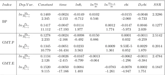
Table 10: The Empirical Evidence on the Optimum Financing Model with Other Indexes – IV

Results: 1974-1997.a b

Index Dep.V ar. Constant time lnθt lnmt_yt lnm_ytt−1 cbi Dtcbi SSR ln_MMt t−1 0.1469 -0.0024 -0.0149 0.0102 -0.0155 -0.0046 2.3286 2.345 -2.153 -0.712 0.546 -2.060 -0.733 BP ln_Pt−1Pt 0.1417 -0.0047 0.0114 0.0012 -0.0147 0.0046 0.1277 11.112 -17.193 1.977 1.774 -5.973 2.039 ln_MMt t−1 0.1278 -0.0024 -0.0098 0.0150 0.0001 -0.0011 2.5142 2.233 -2.166 -0.492 0.886 0.032 -0.259 GMT.P ln_Pt−1Pt 0.1345 -0.0051 0.0233 0.0009 9.53E-5 0.0029 0.2014 10.779 -16.434 3.563 1.361 0.052 1.870 ln_MMt t−1 0.1134 -0.0026 -0.0167 -0.0013 -0.0062 -0.0011 2.4784 2.126 -2.415 -0.799 -0.064 -1.296 -0.384 GMT.E ln_Pt−1Pt 0.1520 -0.0050 0.0084 -0.0783 -0.0078 0.0002 0.1847 9.115 -17.166 1.403 -1.261 -4.947 1.751

a _{t-ratios are reported under the corresponding estimated coefficients.}

b _{Instruments are the lagged value of the logarithm of tax rate, the lagged value of the deviation of}

real GDP from trend expressed as a ratio of trend-real GDP, the logarithm of the lagged government spending-GDP ratio, the time trend.

Table 11: Robustness Tests with Other Indexes – IV Results: 1974-1997.a b

Index Dep.V ar. Constant time lnθ_t lnmt_yt lnmt−1_yt cbi D_tcbi lng_t υ_t SSR

ln_Mt−1Mt 0.1552 -0.0030 -0.0383 0.0110 -0.0118 -0.0028 0.0359 2.09E-12 2.1418 2.207 -2.579 -0.531 0.476 -1.010 -0.296 0.415 0.238 BP ln_PPt t−1 0.1329 -0.0048 0.036 0.0016 -0.0180 0.0055 -0.0340 6.24E-12 0.1226 8.751 -17.718 1.882 2.100 -6.908 2.415 -1.519 3.091 ln_Mt−1Mt 0.1405 -0.0029 -0.0331 0.0176 0.0085 -0.0055 0.0408 -4.73E-12 2.3103 2.240 -2.589 -0.454 0.853 1.310 -0.983 0.493 -0.554 GMT.P ln_PPt t−1 0.1477 -0.0005 -0.0266 0.0001 -0.0010 0.0036 0.0503 3.07E-12 0.1990 10.970 -15.630 -1.098 0.199 -0.517 2.199 2.299 1.239 ln_MMt t−1 0.1302 -0.0031 -0.0196 -0.0023 -0.0058 -0.0007 0.0087 1.12E-12 3.8171 2.089 -2.746 -0.256 0.095 -0.858 -0.221 0.098 0.133 GMT.E ln_Pt−1Pt 0.2121 -0.0050 0.0018 -0.0025 -0.0108 0.00173 -0.0071 5.13E-12 0.1797 12.173 -16.737 0.089 -2.855 -5.713 1.917 -0.298 2.270

a _{t-ratios are reported under the corresponding estimated coefficients.}

b _{Instruments are the lagged value of the logarithm of tax rate, the lagged value of the deviation of}

real GDP from trend expressed as a ratio of trend-real GDP, the logarithm of the lagged government spending-GDP ratio, the time trend.

View publication stats View publication stats