Fractionalization effect and government financing

Fractionalization Effect and Government Financing Article · February 2005 Source: RePEc CITATION 1 READS 46 2 authors, including:

Some of the authors of this publication are also working on these related projects:

Energy Economics: Effect of Oil prices on macroeconomic variablesView project

Output Employment RelationshipView project M. Hakan Berument

Bilkent University

145 PUBLICATIONS   1,893 CITATIONS    SEE PROFILE

All content following this page was uploaded by M. Hakan Berument on 03 June 2014. The user has requested enhancement of the downloaded file.

Fractionalization Effect and Government Financing

Hakan Berument

*

and Jac C. Heckelman

Bilkent University and Wake Forest University

Abstract The weak government argument claims that fractionalized governments (coalition or minority governments) have more difficulty increasing their tax revenues or decreasing their spending than majority governments. This implies that weaker governments are associated with higher government deficits. In this paper, we test the implication of a fractionalization effect within the optimum financing model that suggests governments raise both their tax and seigniorage revenues to finance additional spending. We test the hypothesis for a sample of ten OECD countries for the period 1975-1997 and extend the period for the non-EU nations in the sample to cover 1975-2003. The empirical evidence presented here supports a positive relationship between the degree of fractionalization and seigniorage revenue. Our results also suggest that creation of seigniorage revenue is lower under right-wing governments and an independent central bank.

Keywords: Fractionalization effect, optimum government financing, central bank independence,

political orientation

JEL Classifications: E62, E50, H21

Introduction

Much attention has been focused on how different government structures affect a country’s ability to control its budget deficit. Roubini and Sachs (1989a,b) present evidence which suggests fractionalized governments (coalition or minority governments) are saddled with higher deficits. They argue this result holds due to veto power on specific projects and the instability of coalition governments. In essence, these politicians are trapped in a prisoners-dilemma game of non-cooperation and collective pork-barreling. The government as a whole would benefit from lower deficits and thus each politician would be willing to sacrifice his own spending and taxing policies, but only if everyone else would do the same. The result is a level of spending that everyone considers too high and/or taxes too low.

Mankiw (1987) notes that governments ultimately face two choices on financing. Budgets are financed through both taxation and seigniorage revenue. Table 1 shows that an increase in monetary base as a percentage of government’s total revenue can be substantial among OECD nations. Since either revenue choice creates inefficiencies at an increasing rate, an optimizing government will choose to alter both tax and seigniorage revenue to match changes in financing spending. Hence, there must be a positive relationship between tax and seigniorage revenues. Combining Mankiw’s model with the evidence presented by Roubini and Sachs suggests fractioned governments may create more seigniorage revenue than majority governments. Since

the fractionalized governments have more difficulty in raising their tax revenues, seigniorage revenue will increase as a passive response.

Andrabi (1997) offers a theoretical foundation for this “weak government” result. He assumes agents bargain over tax rates, and the Central Bank will automatically fund any budgetary shortfall through seigniorage revenue. This results in a two-stage game where the level of seigniorage is implicitly determined by the tax bargaining solution. Andrabi assumes the agents realize both taxes and seigniorage are distortionary, but each agent bears the full cost of a distortionary tax on a certain product, and the distortions of seigniorage are spread across all agents. In Andrabi’s model, the Nash bargaining solution results in less than the cooperative rate of taxes, and therefore higher than cooperative seigniorage creation, since the agents do not incorporate the externalities of distortionary seigniorage revenue. One implication of the model is that the level of seigniorage is a function of the number of agents. As the number of agents increases, costs are spread over an increasing number of groups, increasing the incentive to engage in more seigniorage revenue. Although Roubini and Sachs (1989a,b) and Andrabi (1997) provide the initial empirical evidence and theoretical foundation for the weak government argument, Grilli et al. (1991) and Sakamoto (2001) could not find supporting evidence on the level of deficit for a set of industrialized countries.

In this paper, we combine the implication of the Roubini - Sachs and Andrabi weak government models with Mankiw’s optimum financing model. We then test the joint model on a panel of ten OECD countries for the period of 1975-1997. Since seigniorage revenue is expected to increase inflation, the optimum financing literature typically uses inflation as a proxy variable for seigniorage (Mankiw 1987, Grilli 1989, Poterba and Rotemberg 1990, Trehan and Walsh 1990). However, inflation is simply a possible by-product of seigniorage creation, and is affected by other factors for which the government will be unable to directly control. Instead, we follow the model developed in Berument (1994), which suggests monetary base growth is a superior proxy for seigniorage revenue. For comparison, we also present results using the standard inflation rate proxy. As it turns out, our results are slightly stronger when using the more traditional inflation proxy.

The political orientation of the government might also determine its sensitivity to generating seigniorage revenue. Partisan theory suggests that right-wing parties are more sensitive to inflation (hence money creation to generate seigniorage) than left-wing parties (Alesina 1988, Alesina and Drazen 1989, Chappell and Keech, 1988). Berument (1994) argues that right-wing governments generate less seigniorage revenue to finance their spending compared to left-wing governments. Hence we consider the political orientation of governments as another factor that affects the optimum financing policies.

Another institutional factor we consider is the degree of central bank independence. In general, the government acts to pressure the central bank to create money either to influence the growth rate of the economy (Alesina 1989, Cukierman 1992) or to finance spending (Berument 1998); those abilities depend upon the independence of the monetary authority. In conjuction with Mankiw’s (1987) optimum financing model, a more independent central bank would constrict the government’s ability to rely upon seigniorage revenue to compensate for any budgetary deficit. Hence, we consider central bank independence as another institutional factor which may influence the seigniorage-tax revenue trade-off.

In the next section, we modify Berument’s (1994) model to include tax rate considerations for fractionalized governments. We then describe the data used to test the weak government hypothesis, followed by the empirical results. The last section summarizes the results.

The Model

A government’s intertemporal budget constraint requires that any change in government debt must be equal to its interest payments for the government debt from the previous period, plus its current spending and minus its tax and seigniorage revenues. A government’s seigniorage revenue is measured as the real change in the monetary base, and seigniorage is calculated as

t t t t t t t _m M M m P M M . 1 1 − − _{= −} − (1)

where is the nominal monetary base (money, hereafter), is the price level and is the

real monetary base at time t . Therefore, a government’s budget constraint can be written as

t M Pt mt t t t t t t t t t m M M y g rb b b (1 1). 1 1 − − − = + − − − − θ (2)

Here b_t is the government debt, g_t is the real government spending, θ_t is the tax rate, is the real income at time t , and

t

y

r is the fixed interest rate.

An optimizing government minimizes its present value of the loss created by taxation and seigniorage revenue to finance its exogenous stream of spending. As in Andrabi (1997), we assume that the economy has commodities and government officials are sensitive to taxes at different levels for each of the products, where

n

n τi is a parameter such that the sensitivity of

taxation for the ith commodity is measured as τiθt at time t . Hence, the loss created by taxation

is measured as . For mathematical tractability, the loss created by seigniorage

revenue is measured as a function of the inverse of the money growth rate. Specifically, the loss is measured as

∑

= + n i t i 1 1 ) ( τ θ α β − − −₍ 1₎1 t t M M .

Let κ be the weight the government assigns to the benefit of the inverse of money

growth and α and β are assumed to be positive constants to indicate that the loss created by

taxation and seigniorage increases at an increasing rate to satisfy the second-order conditions. Hence, the government objective function is the following:

Min

∑

∑

∞ = = − + − + + + − ⎥ ⎥ ⎦ ⎤ ⎢ ⎢ ⎣ ⎡ − + = 0 1 1 1 1 ) ( ) ( ) 1 ( j n i t j j t j t i j t M M r W τθ α κ β (3)

The τ_i’s represent a government’s fixed preferences regarding the distribution of the burden of

taxes among the n commodities, and θt and t t

M

M ₋₁

Solving the optimization problem results in first-order conditions where the marginal loss of taxation is α θ θ τ ε α ⎥ ⎦ ⎤ ⎢ ⎣ ⎡ + +

∑

= n i t i t y (1 ) 1 1 (4)

and the marginal loss of money growth is

) 1 ( ) 1 ( 1 µ β ε κ β − ⎥ ⎦ ⎤ ⎢ ⎣ ⎡ − − − t t t m M M (5)

where ε_θ is the constant elasticity of income with respect to the tax rate, θ_t; ε is the constant _µ elasticity of the real money holdings with respect to the money growth rate,

t t

M

M 1

1− − . These two

elasticities are included into the model to account for the effect of a change in tax rates on income and the effect of a change in monetary base growth on real money holdings. The first-order conditions require that the marginal loss of taxation and money growth must be equal. Therefore, the following equation can be derived after equating the logarithms of equations (4) and (5):

⎥ ⎦ ⎤ ⎢ ⎣ ⎡ + + + ⎥ ⎦ ⎤ ⎢ ⎣ ⎡ + − + − =

∑

= − n i i t t t t t y m M M 1 1 ln ln ln 1 ) 1 ( ) 1 ( ) 1 )( 1 ( 1 ln τ β α θ β α β ε κ β α ε β _θ µ (6)

Equation 6 suggests that there is a positive relationship between the logarithm of the tax

rate (tax rate, hereafter), and the monetary base growth (money growth, hereafter).1 Furthermore,

a higher level of political fractionalization will cause at least one of τ_is to increase because the new party is likely to be sensitive to the tax rate of a particular commodity more than other

members of the coalition government (Roubini and Sachs 1989a). Hence will increase

as suggested by the envelope theorem; it can be shown that higher fractionalization causes higher rates of money growth, ceteris paribus. Since it is practically impossible to determine what will happen to the tax rates for each type of commodity, it will be assumed that higher levels of fractionalization will cause higher levels of disagreement (Andrabi 1997). To be particular, we

proxy with ⎥ ⎦ ⎤ ⎢ ⎣ ⎡

_∑

= n i i 1 ln τ ⎥ ⎦ ⎤ ⎢ ⎣ ⎡

∑

= n i i 1

ln τ ϕ℘_t where℘ is the degree of fractionalization. _t

Equation (6) assumes that any inefficiencies created by taxation and seigniorage revenue are fixed. However, as suggested by Trehan and Walsh (1990), we recognize these inefficiencies may differ across countries and change over time in a non-systematic manner. Thus, to properly capture the relationship between seigniorage revenue and fractionalization, we include a random error component, εt.

t t t t t t t y m M M _{γ γ γ θ φ ε} + ℘ + + + + − ln ln _{1 2 3} 1 (7)

The model suggests that γ₂, γ3 and φ will all be positive. 2

Data

Mankiw’s (1987) optimum financing model implicitly assumes that governments have the means of collecting tax revenues if they wish to raise taxes. Developing countries, however, often lack the infrastructure to collect this source of potential revenue. Hence, we use data from ten OECD countries to test the basic implication of the model. Our main sample includes annual observations for Australia, Austria, Canada, Finland, Germany, Ireland, Japan, Netherlands, the United Kingdom, and the United States, from 1975-1997 which ends prior to adoption of the common currency EURO.

Klein and Neumann (1990) note that revenue created by central banks (change in monetary base) can be used to buy government debt, to lend to the private sector, or to acquire net international reserves. Hence, central banks’ seigniorage revenue creation needs not be equal to the revenue generated to finance government spending. The amount of revenue generated to finance spending at a given level of monetary base depends upon the institutional and operational procedures of central banks. We measure the change in monetary base as a proxy for government seigniorage revenue to finance spending. The reason is that measuring net transfers requires making some arbitrary decisions for each country that makes the comparison of transfers of income to government across countries more difficult. Hence, we used monetary base growth (Berument 1994) and inflation (Mankiw 1987, Poterba and Rotemberg 1990) as proxies for the seigniorage revenue. Furthermore, monetary base growth is an indicator of the governments’ monetary policy. It is also interesting to see how governments’ optimum monetary and fiscal policies are set under different political and institutional factors. The inflation rate is calculated as the first difference of the logarithm of the consumer price index, and the money growth rate is calculated as the first difference of the logarithm of the monetary base. Data for the CPI and monetary base are gathered from the International Financial Statistics published by the International Monetary Fund.

Data on individual country tax rates are proxied by the average tax rate. The weak government model predicts that certain taxes will be lowered under coalition bargaining in order to take advantage of external seigniorage costs, and also lower taxes on certain products will not be compensated by higher taxes on other products. On average, the overall tax rate should be lower. We expect central government receipts to sufficiently proxy for tax revenues. The average tax rate is calculated as the ratio of central government’s receipts to GNP. Central government receipts are available from OECD National Accounts, Income and Outlay Transactions of General Government.

Fractionalization is represented by the number of parties in the government, taken from Sakamoto (2005). This linear scale would lead to a misspecification bias if, as in Andrabi’s (1997) model, the fractionalization effect is ”concave in the number of parties”. Following Edlin and Ohlsson’s (1991) criticism of the Roubini-Sachs linear scale, we also tried using different dummy variables for each level of fractionalization. However, none of these variables were

individually statistically significant (possibly due to the type II error), but were always jointly significant, suggesting a single scale offers a sufficient approximation.

Regression Results

Including both the tax rate and money growth rate in the same regression equation may create a problem. Each of these series may follow a time trend. Simple regression analysis may capture the time trend they share rather than the underlying relationship we are looking for. To capture this effect, we include a time trend, as Mankiw (1987) and Poterba and Rotemberg (1990) did when analyzing inflation rates.

Including tax rates as an independent variable leads to another methodological problem. Classical regression analysis requires all the independent variables to be exogenous. The Mankiw and Andrabi models imply that tax rates and seigniorage revenue are simultaneously determined. In this case, Ordinary Least Squares estimates are biased. To account for this problem, we use an instrumental variable (IV) approach, using the time trend, the lag value of logarithm of tax rates, lag value of deviation of real GNP from time-trend real GNP ratio, logarithm of lagged ratio of

government spending3 to GNP, lagged monetary base growth and inflation rate, and the

fractionalization variable.

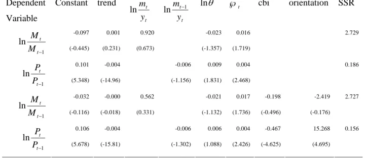
Estimates of the second stage instrumental variable regressions are listed in Table 2. We report the estimates for regressions using both money growth and inflation as the dependent variables.

The first two rows report estimates of the basic model. The estimated coefficient of the

tax rate is not statistically significant4 when the dependent variable is money growth, but is

positive and significant when the dependent variable is the inflation rate. This partially supports Mankiw’s (1987) argument that as governmental spending increases, they make use of both taxes and seigniorage revenue. The estimated coefficients for the coalition variable are positive and statistically significant at the 10% level for money growth and at the 1% level for inflation, thus supporting the weak government model and linear scale utilized by Roubini and Sachs (1989a).

Berument (1994, 1998) argues that the seigniorage-tax revenue relationship alters across countries with the orientation of the governments and different levels of central bank independence (CBI). The second panel of Table 2 repeats the analysis by including a dummy variable for the orientation of the governments (orientation), coded as 0 for right-wing and 1 for left-wing governments, as classified by Sakamoto (2005), and the CBI index from Cukierman (1992). The results on the estimated coefficients for the original variables remain robust to their inclusion. The estimated coefficients for these new variables are not found to be significant in the money growth regression but are significant and have the expected sign in the inflation regression.

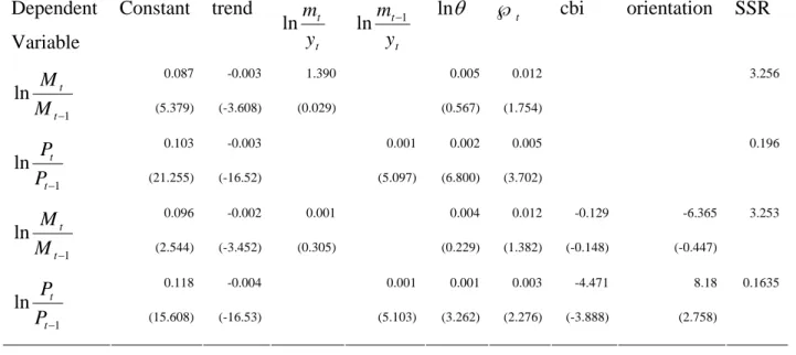
Two countries in our sample may present additional difficulties. The unification of Germany in 1989 may affect the stability of their time series data, and the United States is unique among the OECD nations in having a presidential system with an independently elected legislature rather than the proportional representation parliamentary system of the other nations. Dropping these two nations from our sample, however, does not substantively alter the results. As mentioned above, one of the reasons we end the sample in 1997 was due to the adoption of single

currency EURO for the some of the countries in our sample.5 We extend the data set through

2003 for the non-Euro countries in our sample.6 These countries are Australia, Canada, Japan, the

set given in Table 2 for the unbalanced extended data and report these results in Table 3. We first note that the estimated coefficients for the tax rate are positive for all the specifications used in Table 3; and these coefficients are statistically significant when the inflation rate is the dependent variable. Parallel with Table 2, the estimated coefficient for the coalition dummy is always positive and statistically significant when the dependent variable is the inflation rate. The estimated coefficients for the central bank independence and the political orientation have the same signs as in Table 2; and the estimated coefficients are statistically significant when the inflation is the dependent variable. In sum, the estimates using the extended sample are robust for money growth, and lend even greater support to the model when using inflation as the proxy for seigniorage.

Summary

This paper tests the implication of the weak government hypothesis within the optimum financing model in an instrumental variable regression framework. We use a panel data set of ten OECD countries for 1975-1997 and extend the sample period for the five non-EU countries to cover 1975-2003. We find fractionalized governments rely on more seigniorage revenue to finance their spending, when seigniorage is proxied by either money growth or inflation. Moreover, the reliance on seigniorage revenue creation, as determined by the rate of inflation, is lower if the country has a more independent central bank or right-wing government, but is unaffected by these institutional considerations as determined by the money growth rate.

Appendix: Derivation of the Inflation-Tax Rate Relationship

A government minimizes its objective functions with respect to its intertemporal budget constraint. The minimization problem of a government is the following:

Min

∑

∑

∞ = = − + − + + + − ⎥ ⎥ ⎦ ⎤ ⎢ ⎢ ⎣ ⎡ − + = 0 1 1 1 1 ) ( ) ( ) 1 ( j n i t j j t j t i j t P P r W τ θ α κ β (8) subject to ) ( ) 1 ( 1 ₁ 1 − − − + − − − + = _t t t t t t t t t m P P m y G b r b θ (9)

where all variables retain the definitions as described in the model section. The marginal loss of taxation is found as α θ θ τ ε α ⎥ ⎦ ⎤ ⎢ ⎣ ⎡ + +

_∑

= n i t i t y (1 ) 1 1 (10)

β η κ β − − − − ⎥ ⎦ ⎤ ⎢ ⎣ ⎡ − ) 1 ( ) 1 ( 1 1 t t t m P P (11)

Here, ε_θ is the elasticity of income with respect to the tax rate, θ_t, and η is the elasticity of real holdings with respect to the nominal interest rate. The following equation can be derived after equating the logarithms of equations (10) and (11).

⎥ ⎦ ⎤ ⎢ ⎣ ⎡ + + + ⎥ ⎦ ⎤ ⎢ ⎣ ⎡ + − + − =

∑

= − − n i i t t t t t y m P P 1 1 1 ln ln ln 1 ) 1 ( ) 1 ( ) 1 )( 1 ( 1 ln τ β α θ β α β ε κ β α η β _θ (12)

Equation 12 suggests that there will be a positive relationship between the logarithms of the tax and inflation rates. Furthermore, there will be a negative relationship between fractionalization

and the inflation rate because higher fractionalization will cause at least one of the τ_is to

increase.

To test the hypotheses the following equation is estimated.

∑

= − − + ℘ + + + = 3 1 ' ' 3 1 ' 2 ' 1 1 ln ln ln i t it i t t t t t y m P P _{γ γ γ θ φ ε} (13)

We expect the estimated coefficients γ₂', ´ γ₃' and φ' to be positive.

Footnotes

* The lead author wishes to thank Anwar El-Jawhari, James Friedman, Michael K. Salemi and Roger N. Waud for their helpful comments and especially appreciates the suggestions of Richard T. Froyen, William R. Keech and William R. Parke. We would like to thank Takayuki Sakamoto for providing the data on political factors.

1. Equations (4) and (5) must hold for all periods. This has random walk implications for both tax and money growth rates (see Trehan and Walsh 1990). In this paper we focus on how fractionalization affects the tradeoff between tax and seigniorage revenues. The implication of fractionalization on the time-series properties of money growth rate and tax rate are left for further studies.

2. The literature on the government’s optimum financing typically assumes that inflation is a suitable proxy for the seigniorage revenue rather than the monetary base growth variable that we use. In the appendix we derive the implications of the basic model of this paper when inflation is used as a proxy for seigniorage and test the implications alongside the monetary base regressions in the Regression result section.

3. The government expenditure figures for Japan and U.S. are not available from the International Monetary Funds- International Financial Statistics tape for the sample periods. This series is taken from OECD National Accounts, Income and Outlay Transactions of General Government for Japan and from the Department of Commerce, Bureau of Economic Research for the U.S.

4. The level of significance is at the 5% level, unless otherwise mentioned.

5. Although the EURO was adopted by most countries in 1999, these countries were forced to abandon implementing their monetary policies independently even before 1998. Thus our sample ends in 1997.

6. The political variables from Sakamoto (2001, 2005) were updated by reviewing various issues of Keesing’s Record of World Events.

References

Alesina, A. 1988. “Macroeconomics and Politics,” Macroeconomic Annual 1988, Cambridge,

MA: MIT Press.

___________. 1989. “Politics and Business Cycles in Industrial Democracies,” Economic Policy, 0(8), 55-98.

___________ and A. Drazen. 1991. “Why are Stabilizations Delayed?” American Economic

Review, 81(5) 1170-88.

Andrabi, T. 1997. “Seigniorage, Taxation and Weak Government,” Journal of Money, Credit,

and Banking, 29(1), 106-126.

Barro, R. J. 1982. “Measuring the Fed’s Revenue from Money Creation,” NBER Working Paper

0883.

Berument, H. 1994. “The Political Parties and Optimum Government Financing: Empirical

Evidence for Industrialized Economies,” Southern Economic Journal, 61(2), 510-519.

__________. 1998. “Central Bank Independence and Financing Government Spending,” Journal

of Macroeconomics, 20(1), 133-151.

Cukierman, A. 1992. Central Banks Strategy, Credibility, and Independence: Theory and

Evidence, MIT Press, Cambridge, Mass.

Edlin, P.-A. and H. Ohlsson. 1991. “Political Determinants of Budget Deficits: Coalition

Effects Versus Minority Effects,” European Economic Review, 35(8), 1597-1603.

Grilli, V. 1989. “Seigniorage,” in Europe in Marcello De Cecco and Alberto Gionannini eds. A

__________, D. Masciandaro, and G. Tabellini. 1991. “Political and Monetary Institutions and Public Financial Policies in the Industrial Countries,” Economic Policy, 6(2), 341-392.

Klein, M. and M. J. M. Neumann. 1990. “Seigniorage: What Is It and Who Gets It?”

Weltwirtschaftliches Archiv, 126(2), 205-221.

DeKock, G. and V. Grilli. 1993. “Fiscal Policies and the Choice of Exchange Rate Regime,”

Economic Journal, 103(417), 347-358.

Mankiw, N. G. 1987. “The Optimal Collection of Seigniorage: Theory and Evidence,” Journal

of Monetary Economics, 20(2), 327-341.

Poterba, J. M. and J. Rotemberg. 1990. “Inflation and Taxation with Optimizing

Governments,” Journal of Money, Credit and Banking, 22(1), 1-18.

Roubini, N. and J. D. Sachs. 1989a. “Political and Economic Determinants of Budget Deficit in

the Industrial Democracies,” European Economic Review, 33(5), 903-938.

__________ and __________. 1989b. “Fiscal Policy,” Economic Policy, 0(8), 99-132.

Sakamoto, T. 2001. “Effects of Government Characteristics on Fiscal Deficit in 18 OECD

Countries, 1961-1998,” Comparative Political Studies, 34(5), 527-554.

__________. 2005. “Economic Performance of ‘weak’ Governments and Their Interaction with the Central Bank and Labor: Deficit, Economic Growth, Unemployment, and Inflation, 1961-1998,” European Journal of Political Research, forthcoming

Trehan, B. and C. E. Walsh. 1990. “Seigniorage and Tax Smoothing in the United States,

Table 1: Seigniorage: Average 1975-1997 (Percentages) Country _{Seigniorage†} Australia Austria Canada Finland Germany Ireland Japan Netherlands United Kingdom United States 2.42 1.61 1.61 2.49 1.79 1.73 5.11 1.22 0.91 2.17

† Seigniorage is defined as the ratio of change in monetary base to total government revenues, excluding the change in monetary base (see the data section for the sources of the data).

Table 2: Seigniorage - Tax Rate Trade-off: 1975-1997.† Dependent Variable Constant trend t t y m ln t t y m 1 ln − ln θ ℘ t cbi orientation SSR -0.097 0.001 0.920 -0.023 0.016 2.729 1 ln − t t M M (-0.445) (0.231) (0.673) (-1.357) (1.719) 0.101 -0.004 -0.006 0.009 0.004 0.186 1 ln − t t P P (5.348) (-14.96) (-1.156) (1.831) (2.468) -0.032 -0.000 0.562 -0.021 0.017 -0.198 -2.419 2.727 1 ln − t t M M (-0.116) (-0.018) (0.331) (-1.132) (1.736) (-0.496) (-0.176) 0.106 -0.004 -0.006 0.006 0.004 -0.467 15.268 0.156 1 ln − t t P P (5.678) (-15.81) (-1.302) (1.088) (2.426) (-4.625) (4.695)

Table 3: Seigniorage - Tax Rate Trade-off: 1975-2003.† Dependent Variable Constant trend t t y m ln t t y m ₁ ln − ln θ ℘ t cbi orientation SSR 0.087 -0.003 1.390 0.005 0.012 3.256 1 ln − t t M M (5.379) (-3.608) (0.029) (0.567) (1.754) 0.103 -0.003 0.001 0.002 0.005 0.196 1 ln − t t P P (21.255) (-16.52) (5.097) (6.800) (3.702) 0.096 -0.002 0.001 0.004 0.012 -0.129 -6.365 3.253 1 ln − t t M M (2.544) (-3.452) (0.305) (0.229) (1.382) (-0.148) (-0.447) 0.118 -0.004 0.001 0.001 0.003 -4.471 8.18 0.1635 1 ln − t t P P (15.608) (-16.53) (5.103) (3.262) (2.276) (-3.888) (2.758)

t-statistics are reported under the corresponding coefficients in parenthesis.

View publication stats View publication stats