E L S E V I E R Operations Research Letters 19 (1996) 87-94
An algorithm based on facial decomposition for finding the efficient
set in multiple objective linear programming
S e r p i l S a y l n
Bilkent University, Management Department, Faculty of Business Administration, 06533 Bilkent, Ankara, Turkey Received 1 January 1995; revised 1 July 1995
Abstract
We propose a method for finding the efficient set of a multiple objective linear program based on the well-known facial decomposition of the efficient set. The method incorporates a simple linear programming test that identifies efficient faces while employing a top--down search strategy which avoids enumeration of efficient extreme points and locates the maximally efficient faces of the feasible region. We suggest that discrete representations of the efficient faces could be obtained and presented to the Decision Maker. Results of computational experiments are reported.
Keywords." Multiple objective linear programming; Vector maximization; Efficient faces; Efficient set
1. Introduction
Given a nonempty polyhedral set X defined as X = { x E ~ n I Ax < b , x > 0}, w h e r e A is an m × n m a t r i x a n d b E R m , a n d a p × n m a t r i x C o f objective function coefficients where p > 2, we can define the Multiple Objective Linear Programming problem (MOLP) as follows:
(MOLP) Maximize Cx, subject to. x E X. Throughout the paper we employ the following notation: For two scalars a and b, a < b denotes a < b o r a - - b . For two vectorsx, y E ~n, x < y denotes xi < yi for i = 1...n, and x~<y denotes
x < y b u t x ~ y .
Incorporation of p objective functions simultane- ously into the linear programming framework ne- cessitates the consideration of efficient solutions for problem (MOLP).
Definition 1. x ° E ~n is an efficient solution for prob- lem (MOLP) i f x ° E X and there exists no x E X such that Cx >~ Cx °.
Let XE denote the set of all efficient solutions for prob- lem (MOLP). The vector maximization approach to problem (MOLP) is based on the assumption that the Decision Maker (DM) prefers more to less in each ob- jective. Therefore XE contains all the relevant trade-off information to be conveyed to the DM. Thus vector maximization algorithms aspire to find all of XE and present it to the DM. (For an overview of alternative approaches to problem (MOLP), the reader is referred to, for instance, [7, 10, 14] and references therein.)
It has been shown that the efficient set for prob- lem (MOLP) can be represented as a union of effi- cient faces of X [15]. However, finding all of XE is a computationally-demanding problem. Furthermore, presenting XE to the DM is a difficult task since it is usually a nonconvex continuous set. Thus most 0167-6377/96/$15.00 Copyright (~) 1996 Elsevier Science B.V. All rights reserved
88 S. Saym/Operations Research Letters 19 (1996) 87-94 vector maximization methods have directed their ef-
fort to finding the set of all efficient extreme points of X (see, for instance, [9, 11]).
Typically, most of the vector maximization al- gorithms suggested for problem (MOLP) follow a "bottom-up search". That is, effÉcient faces are gen- erated based on the information provided by efficient extreme points by incorporating certain tests (see, for instance, [8, 12]). Recently, Armand and Malivert [2] and Armand [1] presented such algorithms and reported computational results. A partial exception to the bottom-up search approach is the method of Yu and Zeleny [15] where a "top-down" search strategy is incorporated into the procedure without giving up the bottom-up search.
Since efficient extreme points are zero-dimensional faces, their number could be expected to be much more than the number of maximally efficient faces due to the combinatorial nature of the problem assuming that maximal efficient faces are of high dimensionality (see Remark 3 in Section 2). It has also been discussed that X may "collapse" under the mapping C, and the structure of the efficient set in outcome space may be much simpler than in decision space. Recently, Dauer and Gallagher [6] have shown that maximally effi- cient faces of X and maximally efficient faces in the outcome space are in one-to-one correspondence, sup- porting the hypothesis that the structure of XE when considered as a union o f maximally efficient faces directly could be relatively simple.
Developing a method for finding maximally effi- cient faces of X by employing a top-down search, that is, by avoiding the generation of lower dimensional efficient faces including efficient extreme points may be a viable idea. Discrete representations of the indi- vidual faces could then be obtained and presented to the DM [4].
In this paper, we propose an algorithm for locating X" E for problem (MOLP). We base our method mostly on the results presented in [15]. Our algorithm dif- fers from the method presented in [15] mainly in its disregarding of the efficient extreme points of X, and in the test employed to detect efficient faces. We use the characterization of faces as a collection of indices that correspond to the constraints holding as equal- ity at that particular face [15]. Thus the problem of searching for maximal efficient faces can be reduced to the problem of searching for collection of indices that
correspond to maximal efficient faces. Therefore a search is performed over the space of collection of indices by employing a simple test that identifies effi- cient faces. Since the search procedure considers faces of possibly higher dimension prior to those of lower di- mension, the obtained solution consists of maximally efficient faces of X.
The purpose of this paper is twofold. First, we want to formulate a method that is easy to understand and implement to find XE. By means of the facial decom- position and the top-down search approach, we aspire to synchronize the vector maximization problem with problems of discrete nature that arise in various other contexts for which search techniques are utilized. Sec- ond, we want to gather empirical information about the structure Of XE and observe its sensitivity to certain factors such as the number of objectives, the number of variables and the number of constraints. The paper is organized as follows. In Section 2, we establish the theoretical background and state our results. Section 3 contains the algorithm. In Section 4, computational results are presented.
2. Problem definition and theoretical background Let F be a subset o f X. F is a face of X if every line segment in X with a relative interior point in F has both end-points in F [13]. A face F is an efficient face if all the elements o f F are efficient. A face F is a maximally efficient face i f F is an efficient face and there exists no efficient face of X that contains F as a strict subset. Let
E
and
where In is the n x n identity matrix and 0 E En. Note that we can now rewrite X = {x E ~n[~X ~ b}. L e t M = {1 . . . m + n } a n d , / g = {I ] I C M } . Define .~l as the matrix derived from ,4 by deleting rows of ,4 not in I. Define /~J as the vector derived from/~ by deleting elements of/~ not in 1. For I E Jg, define F(1) = {x E X I Alx =/~z}. For I E ~ ' , F(1) represents a face of X [15]. Note that, F ( 0 ) = X and for I E J / , F ( I ) = (~ is possible. We will refer to F(I) as a proper face o f X i f F ( I ) ¢ ~).
S. Saym I Operations Researc :h Letters 19 (1996) 87-94 89 The following observations about the characteriza-
tion, some of which are given in [ 151, will be useful in understanding the algorithm.
Remark 1. Given a face of X, its representation by F(Z) may not be unique. In other words, for Z, J E Jlt such that Z # J, it is possible to have F(Z) = F(J).
Remark 2. Let 111 denote the number of elements of I. If 111 s JJ(, then dim(F(Z)) zdim(F(J)). Indeed, in the absence of degeneracy, for )I) > n, F(Z) = 0 and for ]I) 5 n, dim(F(Z)) = n - (I].
Remark 3. The number of faces of X of dimension k is bounded from above by the quantity
(n+m)! = (n - k)!(m + k)!
Remark 4. If Z C J, then F(J) &F(Z).
The following results will help us identify those F(Z) that are efficient. First, for Z E A, define the problem (SPI)
(SPt) VJ = max : erCx - erCy, (1)
s.t. r?x 5 6, (2)
Jy 5 6, (3)
jly = &‘, (4)
-cx+cy 5 0, (5)
where x E Iw” and y E W.
Proposition 1. Let Z E A%‘. F(Z) is aproperface of X
tf and only ifproblem (SPI) has a feasible solution.
Proof. (i) Assume that F(Z) is a proper face of X. Then there exists a point y E F(Z). By definition of F(Z), y satisfies Ay 5 6 and A’y = 6’. Let x = y. Then (x, y) constitutes a feasible solution for problem (SPI ).
(ii) Assume that problem (SPI) has a feasible solution (x, y). Then, by (3) and (4), y E F(Z). Thus F(Z) is a proper face. 0
Theorem 1. Let Z E A. F(Z) is a proper efJicient
face of X if and only if the optimal objective function value vt exists and is equal to 0.
Proof. (i) Suppose that F(Z) is a proper efficient face of X. Assume, to the contrary, that the optimal objec- tive value VI for problem (SPI) does not exist or is not equal to 0.
Case 1: vt does not exist. Since F(Z) is a proper face, problem (SPl) has a feasible solution by Propo- sition 1. Thus VI does not exist implies that prob- lem (SPI) is unbounded. This implies that there exists y E F(Z) (by (3) and (4)) and x E X (by (2)) such that Cx 2 Cy (by (5)) and eTCx - eTCy > 0 (by (1)). This implies that Cx 2 Cy. Thus y E F(Z) is not efficient, which contradicts the supposition that F(Z) is an efficient face.
Case 2: VI # 0. Observe that VI > 0 should hold since for any y E F(Z), (x, y) with x = y is a feasible solution for problem ( SPI) and results in an objective value of 0. Then, by an argument similar to that in Case 1, there exists y E F(Z) and x E X such that Cx 2 Cy, which contradicts the supposition that F(Z) is an efficient face.
(ii) Suppose that VI exists and is equal to 0. Then there exists no x, y E [w” that satisfies (2H5) with eTCx > eTCy. Then for all x E X and y E F(Z) such that Cx 2 Cy,
cx = cy (6)
holds. Since F(Z) # 0, we can pick any y E F(Z). Then by (6), there exists no x E X such that Cx > Cy. Hence y E Xs follows. Since y E F(Z) was chosen arbitrarily, it follows that F(Z) is an efficient face of x. 0
Let .,#Yk = {I E & 1 IZ) = k} fork = 0, 1, . . , m+n. Since & = UrLl Ak, it follows that (cf. Theorem 4.1 in [15])
??+?I
XE=
(_j
u
&nF(Z). k=O IE&(7)
Since X, n F(Z) = F(J) for some J 2 Z ([ 15]), there exists b” C A”, 8’ & Ai,. . . &“‘+” & &Pin such that
m+n
XE =
u
u
F(Z).k=O I&
(8)
Note that, by Remark 1, 6, k = 0,. . . , m + n, need not be unique. However, based on (8), it is possible
90 S. Saym I Operations Research Letters 19 (1996) 87-94
to formulate an algorithm that identifies XE by identi- there are no more index sets in ~/¢ to be processed. A fying d 'k, k = 0 .... , m + n. formal description of the algorithm is given below.
3. The algorithm
3.1. The aloorithm statement Step 0 0.0
The proposed algorithm for finding XE is based on checking elements of ~¢k starting with k = 0. For
0.1 k = 0, the only element of J t 'k is 0 and F ( 0 ) = X.
Thus, by solving problem (SP0), the algorithm first
checks if problem (MOLP) is completely efficient Step I 1.0 or not [3]. If problem (MOLP) is completely effi-
cient, the algorithm terminates with the conclusion
XE = X. If not, then for each element I of ~t '1, 1.1 problem (SP1) is solved. If problem (SP1) is infea-
sible, I is dropped from further consideration since
F(I) = 0 (by Proposition 1), and is placed in a 1.2 list that keeps index sets yielding infeasible combi-
nations. If problem (SP1) has an optimal objective
value of 0, I is dropped from further consideration 1.3 since F(I) is efficient (by Theorem 1). In this case,
I is placed in a list that keeps index sets yielding 1.4 efficient faces. If problem (SP1) is unbounded or has
a positive optimal objective value, we can conclude that F(I) has at least one element that is not effi- cient. Therefore, it is possible to have F ( J ) C F(I)
efficient and thus J D I should be checked via solv- 3.2. Validation
ing problem (SPj). Hence, immediate supersets of I, i.e., index sets that contain I and belong to ~t '111+1, are placed in a list for later consideration.
After all the elements of ~¢/1 are considered, the XE = ] [ F(I). index sets that were placed in the list are consid- ieg.~ ered in the order they were placed in the list. For
an index set I, first it is checked if it is a super- set of an index set previously placed in the list of infeasible index sets. If so, I is also an index set that yields an infeasible combination by Remark 4 and therefore is discarded. Next it is checked if I is a superset of an index set previously placed in the list of index sets that yield an efficient face. If so, I is also an index set yielding an efficient face that is a subset of a previously identified efficient face by Remark 4 and therefore is discarded. If these tests fail, then problem (SPI) is solved and I is placed in an appropriate list based on the re- sult obtained from the solution of the linear pro- gram as described above. The procedure stops when
Set I = 0. Solve problem (SPj). If v / = 0, then X = X~. Set 8L~' = {0} and STOP. Else, go to step 0.1. Set k = 1,gL, e = O, J L P = O, La = d ¢ 'k, and go to Step 1. If LP f~ J t 'k = 1~, set k = k + 1. If k = m + n + 1 or £P N jCk = 0, STOP. Else, pick I c Le fq ~gk.
If I ~ J for some J E JL~' or I ~ J for some J G g6q, set ~ = ca \ {i} and go tc 1.0. Else solve problem (SPI).
If problem (SP~) is infeasible, set J L P = u set = \ { I } .
Go to 1.0.
If vl = O, set gLP = g ~ U {I}, set £P = £P \ {I}. Go to 1.0.
Set ~ = &a \ {i} U j l , where j l denote, supersets of I that belong to J t 'k+l. Go to 1.0.
To validate the algorithm, we need to show that
By construction, g&a contains index sets I such that problem (SPt) has an optimal objective value of 0. Thus ATE D UIEt.~ F(I) is obvious by Theorem 1.
To see XE C_ U/Et.~' F(I), it is necessary to observe that all elements of ~ are inspected by the algorithm explicitly or implicitly. Indeed, a search procedure is conducted over ~g by considering elements I in the order of nondecreasing cardinality (Step 1.0) to iden- tify those elements that correspond to efficient faces of X. Note that £P is initialized to ~¢1, and whenever an element I is removed from LP, its immediate supersets are added to L~ (Step 1.4) unless it is guaranteed that
F(I) = 0 (Step 1.2) or F(I)C_XE (Step 1.3). Thus, by (7) and Step 1.3, it follows that XE C_ UI~g.~ F(I).
3.3. Implementation issues
r({1}) A crucial part of the algorithm is keeping various
lists of sets of discrete elements. To increase the efficiency o f the list-keeping procedures, it is possible to consider I E ~ as an (m + n)-tuple
~I = (~1 . . . ~(m+,)) such that ~i = 1 1 1 1 if i E I, and 0 otherwise. Thus it becomes possible to avoid dupli- cate evaluations of index sets by following a lexico- graphic order o f ~I,s in the processing of the list A a and in generation of j 1 in Step 1.4.
In addition to list-keeping schemes, the only re- quirement to implement the algorithm is a tool to solve the linear programming problems. This re- quirement can be met, for instance, by utilizing the simplex method, which is simple and easy to imple- ment. Furthermore, the following observations can be made regarding the use o f simplex method in the algorithm.
(1) When solving problem (SPt) for I E d,/, if the objective value is detected to be positive at any iteration, there is no need to solve the problem to optimality since it is guaranteed that vt > 0 or problem (SPi) is unbounded, and F ( I ) is not an efficient face.
(2) For J E j i , problem (SPs) differs from problem (SPt) in only one constraint. Therefore, the solu- tion to problem (SPz) can be used as a starting solution for problem (SPj). This could possibly improve computational performance.
It can be noted that the proposed algorithm does not require an explicit treatment o f degeneracy and un- bounded feasible region since it does not concentrate on efficient extreme points or efficient bases. Thus by avoiding complex book-keeping schemes, it remains simple and easy to implement.
3.4. An example
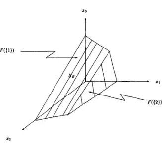
Consider the problem (MOLP) with
1 , C = 1 and b = 8 " 0
The efficient set is the union o f the two maximally efficient faces that correspond to I1 = { 1 } and 12 = {2} (see Fig. 1). Here, M = { 1 .. . . . 5}. The algorithm proceeds as follows.
Z3
X2
Xl
F({2})
S. Sayml Operations Research Letters 19 (1996) 87-94 91
Fig. 1. Example: X and XE.
0.0 Solve problem (SP1) with I = O. vt > O.
0.1 k = 1,8£# = 0,Y.LP = 0,La = {{1},{2},{3}, {4},{5}}.
1.1 Solve problem ( SPz ) with I = { 1 }.
1.3 vz = 0. g£# = {{1}},La = {{2},{3},{4},{5}}. 1.1 Solve problem (SPt) with I = {2}.
1.3 /)I = 0. ~ . ~ = {{1},{2}},.LP = {{3},{4},{5}}. 1.1 Solve problem (SP~) with I = {3}.
1.4 LP = {{4},{5},{3,4},{3,5}}. 1.1 Solve problem
(SPI)
with I = {4}. 1.4 L~ ° = {{5},{3,4},{3,5},{4,5}}. 1.1 Solve problem (SP1) with I = {5}. 1.4 L# = {{3,4},{3,5},{4,5}}.1.1 Solve problem
(SPI)
with I = {3,4}, (k = 2 in Step 1.0).1.4 £P = {{3,5},{4,5},{3,4,5}}. 1.1 Solve problem (SPI) with I = {3,5}. 1.4 ~ = {{4,5},{3,4,5}}.
1.1 Solve problem
(SPI)
with I = {4,5}. 1.4 £P = {{3,4,5}}.1.1 Solve problem (SPI) with I = {3,4,5}, (k = 3 in Step 1.0).
1.4 & a = 0 .
1.0 k = 4, ~e N ~¢/k = 0. STOP.
4. Computational results
In this section we present our computational ex- perimentation with the algorithm. The algorithm was coded in C, and the CPLEX Callable Library [5]
92 S. Saym/ Operations Research Letters 19 (1996) 87 94
Table 1
Computational results:CPU and primary storage requirements
CPU time (seconds) Total LP pivots Working list size Infeasible list size p x m x n Min. Avg. Max. Min. Avg. Max. Min. Avg. Max. Min. Avg. Max.
03 × 10 × 03 a 0.2 0.3 0.3 26 71.6 112 8 14.4 22 7 8.4 10 03 × 10 × 03 0.2 0.3 0.4 50 120.2 231 12 21.6 28 8 11.1 15 03 × 10 × 10 203.1 559 1247.7 37803 151825.3 452446 17200 38399.4 77968 30 95.5 203 03 × 15 × 10 237.4 1143.3 2105.9 34187 264859.8 500728 18650 61733.2 105580 64 197.9 399 05 × 10 × 05 a 0.5 1.1 1.9 97 417.8 925 48 92.4 156 6 10.2 19 05 × 10 × 05 1.2 2.4 3.7 373 1150.6 2030 96 179.4 292 8 15.9 22 05 × 10 × 10 201.9 634 1500 35757 202883.8 661551 17112 37960.2 76762 29 95.4 203 05 x 15 × 10 284.5 1224.1 2252.9 65231 332334.8 598421 18268 59108.6 105434 63 191.1 399 07 x 10 x 07 a 3 7.5 12.7 595 2244.7 4071 304 636.2 936 11 15.4 22 07 x 10 × 07 9.4 19.7 29.3 3 2 1 6 7 8 7 6 . 8 15182 604 1293.8 1772 12 25.7 38 07 × 10 x 10 2 1 2 . 2 7 0 0 . 6 1532.8 47454 245629.4 580017 14906 3 6 2 7 7 76572 25 91.9 202 07 x 15 × 10 322.8 1092.3 2327.2 103954 328146.6 617840 17544 4 9 9 5 2 105304 57 162.9 399 a Problems that are solved for admissible points.
was used to solve the linear programming problems (SPt). The computational experiments were con- ducted on a multi-user SunSparc workstation. In our computational experiments, the class of a problem is determined by the n u m b e r of objectives ( p ) , num- ber of constraints (m) and the n u m b e r o f variables (n). For each problem class, we created a set o f 10 test problems. In the test problems, the elements of the constraint matrix A, the right-hand-side vector b, and the objective function coefficient matrix C were randomly generated integers belonging to the discrete uniform distribution in the intervals (1,20), (50, 100) and ( - 1 0 , 20), respectively. A 25% zero density was provided in the matrix A. Nine different classes were constructed according to the values of p, m and n. Three additional problem classes were created by solving the test problems in three categories with p = n for admissible points (i.e., with C = Ip, where
Ip is the p × p identity matrix).
The results of computational experiments are re- ported in two separate tables. The first table contains information regarding the computational performance of the algorithm. Along with CPU times, we report total n u m b e r of LP-pivots as an indicator o f computa- tion time. As an indicator o f storage requirements, the size o f the working list (LP) and the size o f the list of infeasible I ' s ( J S e ) are reported. In Table 1, it can be observed that computational requirements increase rapidly with problem size. It can also be observed that
n u m b e r o f variables seems to have the most signif- icant effect on computation time where the n u m b e r of constraints also seems to be important. Based on these preliminary results, n u m b e r of objectives does not seem to be a very important factor. Another obser- vation is that solving for admissible points is likely to be easier than solving for efficient points, especially as the problems get larger.
Table 2 contains the information pertaining to the structure o f the test problems solved. Basically, it would be interesting to know the n u m b e r o f distinct ef- ficient faces and the dimensions o f each for each prob- lem. As one pseudo-measure, we report the efficient list size (~f~q), which is an upper b o u n d on the n u m b e r of distinct efficient faces (see Remark 1 ). To have an idea about the dimension o f the highest dimensional efficient face, we report Illmin = m i n s e ¢ ~ l I [ , since n - lI[min is a lower bound on this quantity. Note that, in the absence of degeneracy, these are exact values rather than bounds. Finally, as an approximate mea- sure in the variation in the dimensions o f the efficient faces, we report Illmax -- [I[min- The results in Table 2 indicate that the efficient set has a relatively sim- ple structure. The efficient list size, though increasing with problem size, seems to be rather reasonable when the combinatorial nature o f the total n u m b e r of faces is considered (Remark 3). That seems to be more in effect for the set o f admissible points. As far as the dimensions of the efficient faces are concerned, an
S. Saym I Operations Research Letters 19 (1996) 87-94
Table 2
Computational results: Structure of XE.
93
Efficient list size [IImin Illm~x --I11mm
p x m x n Min. Avg. Max. Min. Avg. Max. Min. Avg. Max.
03 x 10 x 03 a 1 2.2 4 1 1 1 0 0.2 1 03 x 10 x 03 I 1.8 3 1 1.6 3 0 0.3 1 03 × 10 x 10 4 11.4 27 8 8 8 0 0.7 1 03 x 15 x 10 4 15.5 45 8 8 8 0 0.6 1 05 x 10 x 05 a 2 3.5 8 1 1 1 0 0.3 1 05 x 10 × 05 1 4.4 9 1 1.9 3 0 0.9 2 05 x 10 x 10 3 25.1 49 6 6.4 8 1 1.8 3 05 x 15 x 10 12 37.3 92 6 6.3 7 1 1.7 2 07 × 10 × 07 a 3 6.4 10 1 1.1 2 0 1 2 07 × I0 × 07 4 12.5 21 2 2.6 4 2 2.2 3 07 x 10 x 10 16 43.6 57 4 4.8 6 2 2.8 3 07 × 15 × 10 16 48.1 93 4 4.7 6 2 3.1 4
a Problems that are solved for admissible points.
Table 3
CPU times (in seconds) for Armand-Malivert test problems
Tube Pyramid Tent
m 20 30 40 50 20 30 40 50 21 31 41 51
0.6 0.9 1.5 2.0 0.6 0.9 1.4 1.8 0.9 1.2 1.8 2.6
important observation is that the variation across the efficient set is rather small. Furthermore, if we take n - II]min as an indicator of the dimension of the high- est dimensional efficient face, for a given value of p, this quantity shows little variation for different values o f m and n. However, more experimentation would be necessary to draw strong conclusions.
In addition to the computational experiments con- ducted, the 12 problems presented by Armand and Malivert [2] were solved for comparison purposes since theirs is the only algorithm with reported com- putational results. The definitions of these problems, where n = 3, p = 2 or p = 3, which possess cer- tain geometrical structures, can be found in [2]. The results are given in Table 3.
The results of computational experiments motivate heuristic modifications of the algorithm. For instance, one may aspire to find efficient faces that belong to a particular set ~gk, where k is determined by finding an appropriate face F(I) E jCk in which an initial
efficient point that has been obtained lies. To see if this type of an approach would generate good results and if it would bring computational benefits requires further study.
References
[1] P. Armand, "Finding all maximal efficient faces in multi- objective linear programming", Math. Programming 61, 357-375 (1993).
[2] P. Armand and C. Malivert, "Determination of the efficient set in multiobjective linear programming", J. Optimn. Theory Appl. 70, 467-489 (1991).
[3] H.P. Benson, "Complete efficiency and the initialization of the algorithms for multiple objective programming", Oper. Res. Lett. 10, 481-487 (1991).
[4] H.P. Benson and S. Sayin, "Finding global representations of the efficient set in multiple objective mathematical programming", Discussion paper, Department of Decision and Information Sciences, Univerity of Florida, 1994.
94 S. Saym/ Operations Research Letters 19 (1996) 87-94
[5] Cplex, Using the Cplex Callable Library and Cplex Mixed Integer Library, Version 2.1, Cplex Optimization, Inc, 1993.
[6] J.P. Dauer and R.J. Gallagher, "A combined constraint-space, objective-space approach for determining high-dimensional maximal efficient faces of multiple objective linear programs",
European J. Oper. Res. 88, 368-381 (1996).
[7] J.S. Dyer, P.C. Fishburn, R.E. Steuer, J. Wallenius, and S. Zionts, "Multiple criteria decision making, multiattribute utility theory: The next ten years", Management Sci. 38(5),
645~554 (1992).
[8] J.G. Ecker, N.S. Hegner and I.A. Kouada, "Generating all maximal efficient faces for multiple objective linear programs", J. Optim. Theory Appl. 30, 353-381 (1980).
[9] J.G. Ecker and 1.A. Kouada, "Finding all efficient extreme points for multiple objective linear programs", Math. Programming 14, 249-261 (1978).
[10] G.W. Evans, "An overview of techniques for solving multiobjective mathematical programs", Management ScL
30, 1268-1282 (1984).
[1 I] J.P. Evans and R.E. Steuer, "A revised simplex method for linear multiple objective problems", Math. Programming 5,
54--72 (1973).
[12] T. Gal, "A general method for determining the set of all efficient solutions to a linear vector maximum problem",
European J. Oper. Res. 1, 307-322 (1977).
[13] R.T. Rockafellar, Convex Analysis, Princeton University
Press, Princeton, NJ, 1970.
[14] R.E. Steuer, Multiple Criteria Optimization: Theory, Computation, and Application, Wiley, New York, 1986.
[15] P.L. Yu and M. Zeleny, "The set of all nondominated solutions in linear cases and a multicriteria simplex method",