i
TURKISH-GERMAN UNIVERSITY
INSTITUTE OF SOCIAL SCIENCES
INTERNATIONAL FINANCE DEPARTMENT
LINK BETWEEN VOLATILITY AND MARKET
ACTIVITY AT DERIVATIVES EXCHANGE EUREX.
MASTER’S DEGREE THESIS
Akın Öğrük
ADVISORS
Asst.Prof Levent Yılmaz
Dr. Michail Koslov
ii
Contents
Contents………ii Dedication.……….……….………....iii Acknowledgement……….….………iv Abstract……….……….…..1 1. Introduction ...2 2. Literature Review...43. Data and Visual Relation Analysis ……….……...…6
3.1 Data Description……….……….6
3.2 Data Visualization………….………….……….7
4. Methodology………...………13
5. Empirical Results and Conclusion……….……..20
6. Reference Page………...22
iii
iv
ACKNOWLEDGEMENT
I would first like to thank my thesis advisors Asst.Prof. Levent Yılmaz
International Finance Department at Turkish-German University and Michail Koslov at Eurex for their supports and valuable feedbacks during this study.
I would also like to thank Gizem Kaya and Hidayet Beyhan at Istanbul
Technical University Management Engineering Department for their help. Whenever I ran into a trouble spot or had a question about my research, they shared their knowledge with me patiently and spent their time for me.
Also, huge thanks to my friends who have tolerated my stressful times and my ‘no’ for their plans. I have not been a good friend during this period but they always respected and understood me.
My family, you are behind of every accomplishment. Nothing would be possible without you.
Author
1
ABSTRACT
LINK BETWEEN VOLATILITY AND MARKET ACTIVITY AT
DERIVATIVES EXCHANGE EUREX
This is a comprehensive study of exploring link between volatility and market actions at Derivatives Exchange Eurex on monthly basis. Study was conducted for both options and futures on 2 volatility types which are actual volatility (based on EuroStoxx 50 Index end of day levels) and implied volatility VSTOXX (EURO STOXX 50 Volatility Index which is based on the real-time market prices of EURO STOXX 50 options) and 2 market actions which are trading volume and open interests. Due to the nature of the end of day index levels, financial data in general, actual volatility has been estimated by using GARCH method. Rest of the data has been directly collected from external sources. Our data includes between January 2007 and August 2019. A regression model has been set and market action has been estimated by lagged market action (1 month lagged), volatility and trend. Results revealed that implied volatility VSTOXX has a strong link with current month’s all type of market activity for both derivatives type while actual volatility, estimated by GARCH model, has only significant relation with option trading volume.
Key Words: GARCH, volatility, VSTOXX, time series, ARMA, derivatives Date:15.07.2020
2
1. Introduction
Derivatives are the financial instruments whose price is derived from underlying asset’s price which can be interest rate, index, stock price, commodities, currency rate etc. Derivatives market plays a significant role in many parts of finance. They have been needed in commerce in the history and we see them practiced in Mesopotamia, Roman Empire, Byzanthian Empire, Italy in renaissance, Antwerp and Amsterdam in the 16th century, England and France at the end of 17th century, and Germany in the early 19th century (Weber 2019, 431). Although there are some more types of
derivatives such as swap and forward, we will only focus on options and futures under the derivatives market in this thesis.
Before going into deep analyzes in the next chapters, let us have a brief information about options and futures. An option is a contract that gives buyers the right, but not the obligation, to buy or sell the underlying asset by a certain date
(expiration date) at a specified price (strike price). There are two types of options: calls and puts. Call options give buyers the right, but not the obligation, to buy the
underlying asset at the strike price specified in the contract. Market players buy call options if they think the price of the underlying asset is going to increase and sell call options if they think it is going to decrease. Put options give the buyer the right, but not the obligation, to sell the underlying asset at the strike price specified in the contract. Put option seller is obligated to buy the asset if the put buyer exercises the option. Market players buy put options if they think the price of the underlying asset is going to decrease and sell puts if they think it is going to increase. There are two exercise styles which are American options, exercisable at any time before expiration date and
European options, only exercisable on the expiration date. Option contracts
are traded either on a public stock exchange or implicitly agreed between buyer and seller also known as Over the Counter (OTC) markets. On the options side, I am going to make use of EuroStoxx options in this study.
Futures are financial contracts which obligate the buyer and seller to transact an asset at a predetermined future date and price. Here, the buyer must buy, or the seller must sell the underlying asset at the specified price, regardless of the current market price at the expiration date. The futures market is centralized, which means they
3 are traded in a physical location or exchange. They are not traded on OTC markets like options. On the futures side, I am going to make use of EuroStoxx futures in this study.
Players in the financial markets generally use derivatives for hedging, speculation and arbitrage purposes. Hedging is generally preferred by risk averse
players to prevent from market risk by fixing the price of underlying asset for the future. We could use analogy between hedging and insurance for better understanding of
hedging. Every year you pay a premium to buy car insurance to get rid of expenses in case of accidents, floods etc. Similarly, options and futures can be used to protect from declining prices of stock market.
Speculation is used by people who want to make profit from short term market movements. They take long or short position and expect market prices either to increase or decrease. It is based on hunches and assumptions, so it involves a significant amount of risk. Speculation is very significant in terms of liquidity. There would be a very limited and illiquid market without speculation activities. Thirdly, arbitrage is a strategy that including the purchase of a security on a market and the sale of it for a slightly higher price on the other market. Arbitrage is not a high risk strategy and it is generally used by hedge funds and large institutional investors.
Although financial guru Warren Buffet says that “derivatives are financial weapons of mass destruction” derivatives highly contribute to the financial markets. Trading of them is vital for financial system members such as fund managers and investors. For investors, trading in derivatives market is magnetic because it empowers them to control of assets with little amounts of money giving the benefit of leverage. Thanks to its low transaction cost it enables investors to have portfolio diversification and hence to reduce the risk. Minimizing risk is possible by taking short and long positions upon the forecast of asset prices in the future. Trading of derivatives is not only minimizing the risk but also increases the liquidity in the market. Introduction of derivatives of the underlying stock augments the opportunity set available to investors and hence brings a positive impact of the liquidity of the underlying stock (Narasimhan et al. 2014).
In this study, I will deeply analyze relation between market activity (open interest and trading volume) of derivatives and underlying stock prices. Here underlying instrument is meant to be EuroStoxx50 index. Trading volume represents the number of
4
contracts completed each day while open interest represents the number of contracts which are held by traders and investors in active positions. Price-volume relation is very crucial for financial markets. There are many interpretations and implications of this relation. For instance, volume information of derivatives may give a clue about the future stock prices. (Pan and Poteshman, 2004) presented that stocks with low put-call ratios performs better than stock with high put-call ratios. In addition, it also gives clue about the liquidity of the stock. (Narasimhan et al. 2014) has found that derivative listing enhanced the liquidity of illiquid stocks significantly.
2. Literature Review
In the earlier literature, we can come across numerous researches about the link between volatility and volume. While many of them inspects the relation between stock price volatility and stock volume, some inspects the relation between stock price
volatility and derivatives’ trading volume. Although they analyze different type of volumes (stock vs derivatives), almost all of them are on shorter time basis such as hourly, daily and weekly instead of monthly basis.
(Cimen 2018) has investigated the spot market volatility after introduction of derivatives for Turkish market. She has applied GARCH method and compared conditional volatility before and after for both futures and options. Results of the GARCH analysis in the paper showed that introduction of derivatives have mitigated spot market volatility. There are some similar studies for the Turkish market (Yilgor, Mebounou 2016), (Baklaci and Tutek 2006), (Çağlayan 2011), which are prior articles and (Cimen 2018) stayed align with these papers in terms of findings. Also, (Kasman and Kasman 2008) which is one of the pioneer studies for Turkish market, used EGARCH model and reached the conclusion that introduction of futures lowers the conditional volatility of ISE 30 index. (Gökbulut et al. 2009) searched impacts of futures trading on spot market volatility only after the introduction of futures. Opposite to other studies, it has been concluded that ISE-30 Index futures contracts has no significant effect on volatility of ISE-30 Index. In terms of structure, my paper looks
5 like (Gökbulut et al. 2009) as they do not measure before and after introduction of derivatives, they just analyze a time period when derivatives are already listed.
(Jeanneu and Micu 2003) has done their research on link between price volatility and derivative’s trading activity. They used S&P500 and Ten-year US Treasury note as assets and they have used the corresponding options’ and futures’ trading activity (trading volume and open interest). They have calculated 2 types of volatility which are called actual and implied volatility. Implied volatility focuses on option’s price while actual volatility focuses on asset’s own price. Since the both option and asset prices follow a time varying pattern, they calculated volatility by GARCH model (Engel 1982) which will be examined in a detailed way in the “Methodology” chapter of my study. Their results revealed that there is a tenuous relationship between volatility and trading activity in monthly basis. This is a contrast to previous research which has been done in daily basis. Even, for 10-year US Treasury note futures and options contracts, the link between volatility and trading volume turned out to be negative. In addition, albeit their different natures, implied and actual volatility have no markedly different impact on trading activity. (Jeanneu and Micu 2003) mainly forms my thesis. I benefited from their methods and it has been a useful guide for my study.
For the other markets worldwide, literature includes contradictory results as well because of the varying volatility calculation methods (non-conditional, ARCH, GARCH etc.), markets, assets and time periods. Numerous of studies analyze introduction of futures’ effects on the volatility of the underlying assets and many of them supports the idea that introduction of derivatives augments the volatility of underlying assets such as (Robinson 1994) on FTSE 100 index by ARCH-M model and S. Bhaumiky, M.
Karanasosy and A. Kartsaklas_on Indian stock market by GARCH model. A few of them suggest that more derivative trading causes to less volatility of underlying assets. A remarkable number of papers find no statistically significance link between those (Edwards 1988) or even finds a negative link (Jeanneau and Micu 2003)
6
3. Data and Visual Relation Analysis Between Price
and Market Activity
3.1 Data Description
As it is mentioned, two types of market activity (trading volume and open interest) will be used for our analysis. Trading volume refers to the measure of contracts traded within a specific time period for a particular asset. It is measured with the number of each transaction, namely every derivative contract traded between buyers and sellers. Open interest can be defined as the number of active derivative contracts for an asset, at a given time point. It represents the positions for a security which have not yet been closed.
Market activity data can be extracted from the following website of derivatives exchange Eurex.
https://www.eurexchange.com/exchange-en/market-data/statistics/monthly-statistics Euro Stoxx 50 is the most commonly traded European equity index, which contains 50 well recognized and large stocks in the Eurozone, such as German Daimler AG and Deutsche Börse, French Airbus, Spanish Inditex, Dutch Philips etc. The VSTOXX indices are based on Euro Stoxx 50 real time options prices and are created to reflect the market expectations of short up to long-term volatility by calculating the square root of the implied variance across options of a given time to expiration (stoxx.com). VSTOXX index provides the implied volatility given by the prices of the options with corresponding maturity, on the EURO STOXX 50 Index (Stanescu and Tunaru,2014). In other words, VSTOXX targets to estimate the volatility of the EUROSTOXX50 index for a future time horizon, as implied by the available option contracts on the Eurex Exchange on that index. Historical data for VSTOXX can be found from below link.
https://www.stoxx.com/document/Indices/Current/HistoricalData/h_v2tx.txt
As mentioned in the abstract, two types of volatilities, VSTOXX and actual, are used in this study. Actual volatility is based on EURO STOXX 50 end of day index levels. I retrieved end of day prices from the following link.
7
3.2 Data Visualization
In this study, link between price volatility and derivatives market activity at derivatives exchange Eurex will be investigated. Study will be conducted monthly basis and contains the publicly available data between Jan 2007 and Aug 2019. Firstly, I have analyzed longer time periods from Jan 2002 to Aug 2019. Yet, below graphs explicitly tell us that derivatives were not intensely traded, and market activity were relatively low in the earlier term. Therefore, I cropped my data and focused on the time between Jan 2007 and Aug 2019 when the market activity is higher. Below 4 tables denote how market activity evolve by time.
Graph 3.1: Trading Volume of Options
8
Graph 3.2: Open Interest of Options
9
Graph 3.4: Open Interest of Futures
In this paper GARCH method is applied to end of day prices. Standard deviation results of the GARCH are accepted as actual volatility. Details of the calculations and models will be inspected in the “Methodology” section. Yet, before moving to modeling, let us visually check some graphs for two types of market activity (open interest and trading volume) and VSTOXX which is ready by Eurex website on two types of derivatives (options and futures). Although I will conduct my empirical work with data between Jan 2007 and Aug 2019, I have used the longer data for visualization. Graph 1 is showing monthly future trading volume with red line and implied volatility (VSTOXX) with blue. As it can be seen, at the beginning where derivatives trading are much lower than the latter periods, relation seems very opposite. Starting from 2005, we realize a similar pattern for futures trading volume and VSTOXX volatility. They increase and decrease together. It is not possible to deduce a causal relationship from this graph but at least we can say that they show a parallelism.
10
Graph 3.5: Futures Trading Volume vs VSTOXX Volatility
Like Graph 1, Graph 2 denotes that trading volume for option and VSTOXX volatility show similar pattern and move up or down together at the same time periods after 2005. Shortly, variables in the first two graphs behaves like they are positively correlated. We can make this conclusion only after 2005 for both graphs. Before 2005, we can interpret that volume for derivatives were relatively low and market had hunger for derivatives. Therefore, even if it has a different direction with volatility, trading volume went up with a market trend. Besides, we observe a sudden peak 2008-2009 in option and future trading volumes. As mentioned in the introduction, one of the common use purposes of derivatives is hedging. Due to the global crisis in 2008-2009 market was too volatile and there was a ambiguous environment. So, this peak may be interpreted as market players’ intention to get rid of the high risk. There may be other reasons for this according to (Chesney 2015) firstly, the high volatility during the crisis leads to fast movements in stock prices which generates opportunities for informed market players; secondly, because of sudden collapse of the system, governmental and corporate decision making have boosted, leading to many information leakages and abnormal trading activities; lastly, trades made before
11 scheduled announcements could be based on speculative bets, the latter being facilitated by some rumors already existed in financial market.
Graph 3.6: Options Trading Volume vs Implied Volatility
Market activity versus volatility graphs were checked and interpreted. Let us have a look at correlation versus market activity graphs. Comment about correlation has been added for the above graphs but below graphs give us opportunity to see the
correlation more clearly. Graph 3.7 illustrates the correlation coefficient between
VSTOXX and trading volume of options and futures. On the left y-axis we see the value of correlation. I used 12 months rolling window while calculating correlation for both Graph 3.7 and Graph 3.8. Correlation is not stable over time. Coefficient is negative only for a few time periods. It is almost positive everywhere other than that time periods and coefficient is generally between 0.4-0.8 which can be accepted as a moderate relation. Also, option trading volume has stronger correlation with volatility than futures trading volume has.
12
Graph 3.7: Correlation of Options and Futures Trading Volume and Implied Volatility
Graph 3.8 shows us, like in the trading volume graph, open interest has positive correlation with volatility for most of the time however correlation is not as strong as in trading volume. We see more time periods where correlation coefficient is negative and as a magnitude it has lower coefficient between 0.25-0.75. In addition, a particular type of derivatives is not dominant in terms of correlation which means sometimes futures sometimes options has stronger correlation. In other words, correlation is not stable over time for open interest of derivative types.
13
Graph 3.8: Correlation of Options and Futures Open Interest and Implied Volatility
4. Methodology
Since we have a volatility time series data represented by VSTOXX index levels and market activity time series data, this study surely has to include time series and statistical analysis. Our method is basically as following; first, I have to make sure all volume and volatility data to be stationary. While calculating the actual volatility best fit ARMA-GARCH model should be determined. After everything is appropriate, a regression model should be set to check the significance of relation between volatility and volume. Let us get into details. You can see below flowchart for following the methodology steps as well.
14
Graph 4.1: Methodology flow chart
All coding for this study has been done in RStudio. You can find the whole code with explanatory comments in the “Appendix” part. Again, our ultimate aim is to search link between volatility and market activity. Therefore, below regression model has been set as in the paper (Jeanneau and Micu 2014).
Market_Activityt =β0 +β1*Trend + β2*Market_Activityt-1 + β3*Volatilityt +
ε
tThis is our generic regression model. We insert open interest and trading volume data into “Market_Activity” variable. ε is our randomly distributed errors and β0 is our
constant for this equation. We insert VSTOXX values or our actual volatility calculated by GARCH model for “Volatility” variable. Lastly, we try these variable types for both options and futures. So, we try this model 2(volatility types) * 2(market activity types) * 2(derivative types) = 8 times for different combinations. Trading volumes, open interest levels and VSTOXX index level data is ready however to be able to use them in the model some tests on the data must be applied. Many statistical forecasting techniques assumes that the time series can be rendered approximately stationary through the use of mathematical transformations. So, it is needed to check the stationarity condition in time series analysis.
Insert all market activity, VSTOXX and end of the day index level data to R
from csv files
Check stationarity of all data and use log transformation and differencing if needed
End of day index level data is visually analyzed
Ljung-Box test is applied to end of the day index level data and GARCH is
applicable Since test is passed, best
fit ARIMA and GARCH models are determined
Coefficients of ARIMA-GARCH model results are
retrieved
Regression model is tried for combinations of VSTOXX&actual volatility,
options&futures, trading volume&open interest.
Results are interpreted, significance between
market activity and volatility is searched
15 A time series basically is stationary if a shift in time doesn’t lead to change in mean , variance and covariance. With more formal definition (Lütkepohl, Krætzig, 2003) A stochastic process yt is called stationary if it has time-invariant first and second
moments. In other words, yt is stationary if
1. E(yt) = µy for all t ∈ T and
2. E[(yt − µy )(yt−h − µy )] = γh for all t ∈ T and all integers h such that t − h ∈ T.
The first condition means that all members of a stationary stochastic process have the same constant mean. Hence, a time series generated by a stationary stochastic process must fluctuate around a constant mean and does not have a trend for instance. The second condition ensures that the variances are also time invariant since, for h = 0, the variance σ2
y = E[(yt − µy ) 2] = γ0 does not depend on t. Moreover, the covariances
E[(yt − µy )(yt−h − µy )] = γh do not depend on t but just on the distance in time h of the
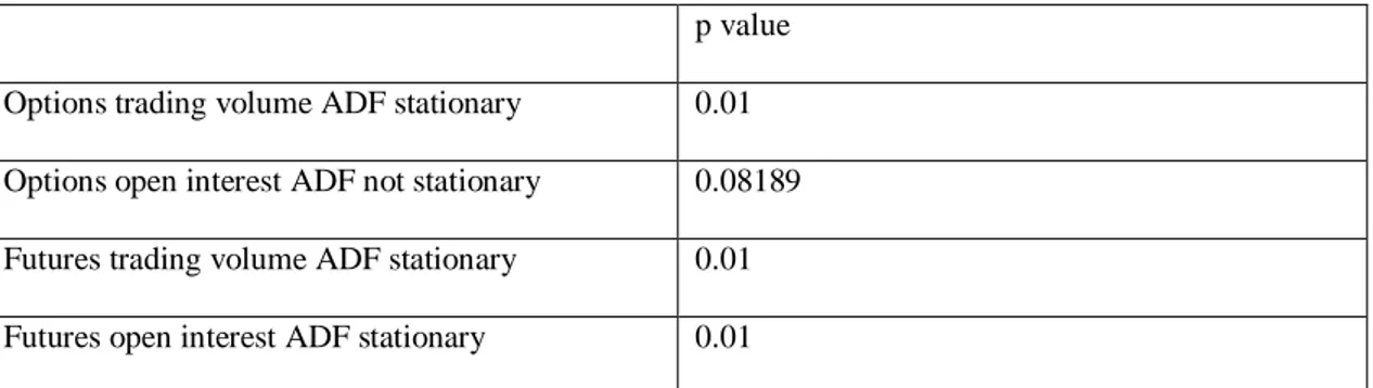
two members of the process. Our notation is also meant to imply that the means, variances, and covariances are finite numbers. In other words, the first two moments and cross moments exist. Firstly, I have applied Augmented Dickey-Fuller test for market activity variables. This test tells us that whether a data set is a stationary or not. Corresponding p-value results are as follows:
p value Options trading volume ADF stationary 0.01 Options open interest ADF not stationary 0.08189 Futures trading volume ADF stationary 0.01 Futures open interest ADF stationary 0.01
Table 4.1: Market activity stationary test before log transformation and differencing So, above results tell us that options open interest data is not stationary, but all of the rest market activity is stationary. There are some methods to transform a
nonstationary series to stationary series and taking difference is one of them.
Differencing of time series is taking the differences between consecutive time periods. Assume that Xt denotes the value of the time series X at period t, then the difference of
16
stabilizing the variance of a series with non-constant variance. This is done by
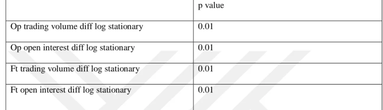
using log() function. Log transformation can be applied only to positively valued time series and our series satisfy this condition. Both methods can be used at the same time with the order first logarithmic transformation then differencing. Since I have a non-stationary data, I have to apply these methods. To be on the safe side I have used both of them to all market activities regardless they are stationary or not. After applying both methods, ADF test results turned out to be as following:
p value Op trading volume diff log stationary 0.01 Op open interest diff log stationary 0.01 Ft trading volume diff log stationary 0.01 Ft open interest diff log stationary 0.01
Table 4.2: Market activity stationary after before log transformation and differencing As we can see from the above test results all market activity data have passed the stationarity test and ready to be inserted into models. I put VSTOXX implied volatility data to ADF test and p-value is 0.01388 which means implied volatility data is stationary. I still used logarithmic transformation and differencing as I did them for market activity data and p-value became 0.01. Till this point all market data and implied volatility data are adjusted and ready for model.
The one which is left is actual volatility. For actual volatility, Euro Stoxx 50 Index end of day levels are going to be used. Like the most financial data, our closing price volatility also carries the similar characteristic in terms of volatility clustering, time varying, conditional volatility. Below table shows us the one period closing price differencing and volatility clustering is so obvious. Volatility clustering means that volatility of a time series is a function of previous levels of volatility, in other words high or low values of volatility are grouped in distinct time periods. Blue circles are the consecutive time periods where volatility clustered with low values and red circles are just the opposite.
17
Graph 4.2: End of day index levels difference
Classical ways of measuring volatility are time invariants measures. However, the variance of stock returns and many other financial data are substantially recognized to be time-varying and, as a natural consequence, time invariant measures stay
inadequate for this kind of data. This ended up with growing effort to improve time-varying methods to model volatility depending on the past values. Widely known models approaching this purpose are ARCH model (developed by (Engle 1982)) After the introduction of ARCH models there has been huge theoretical and practical
improvements in financial econometrics in the 80’s. It turned out that with ARCH models, time series could efficiently be modeled and empirical findings could be easily represented in financial time series. Especially, after the collapse of the pegged
exchange rate system known as Bretton Woods system and the implementation of flexible exchange rates in the 70’s ARCH models are used by researchers and
professionals with accelareted rate. After a couple of years and GARCH (Generalized Autoregressive Conditional Heteroskedasticity) model which represents an extension of the ARCH model into a generalized one has been developed by (Bollerslev 1986).
GARCH models provide the way of modelling conditional volatility. They are useful in situations where the volatility clustering exists. A GARCH model is typically of the following form:
18
which means that the variance (σt)2 of the time series today is equal to a constant (ω),
plus some amount (α) of the previous residual (εt-i), plus some amount (β) of the
previous variance (σt-i)2.
I have applied Ljung-Box test to check whether data is appropriate for GARCH. The Ljung-Box test checks for autocorrelation within the GARCH model’s residuals. If GARCH model suits well to data, there should not be auto-correlation for residuals. On RStudio I applied Ljung-Box Test on end of day stock index data after differencing and logarithmic transformation. Should the p-value be <= 0.05 then we assume that
GARCH model is a suitable model to estimate the volatility. According to test result I find out that p-value equals to 0.0002853 which means we can apply GARCH to this data.
Now it is time to find the best fit model to use for our end of day stock index data. As I said before, GARCH model will be applied but GARCH model is applied together with an ARMA model. ARMA models aim to describe the autocorrelations in the data. In autoregression models (AR), we predict the variable of interest using a linear combination of historical values of the variable. The term autoregression denotes that it is a regression of the variable against itself.
Therefore, an autoregressive model with order p can be formulated as
yt=c+ϕ1yt−1+ϕ2yt−2+⋯+ϕpyt−p+εt
where εt is white noise. This is like a multiple regression but with lagged values of
yt as predictors. We refer to this as an AR(p) model, an autoregressive model of order
p.
Instead of using historical values of the forecast variable in a regression, moving average model uses past forecast errors in a regression-like model.
19
where εt is white noise. We refer to this as an MA(q) model, a moving average model with order q.
To determine best fit p and q values there is a useful auto.arima() function in RStudio. Code output denotes that ARMA (1,1) is the fittest model for prediction. This RStudio function chooses p and q variables by minimizing some criterias which are AIC (Akaike Information Criteria), AICc (Corrected AIC) and BIC (Bayesian Information Criteria). AIC is handy for determining the order of the ARMA model. It is formulated as following;
AIC=−2log(L)+2(p+q+k+1)
where L is the likelihood of the data, k=1 if c≠0 and k=0 if c=0. Note that the last term in parentheses is the number of parameters in the model (including σ2, the variance of the residuals).
For ARMA models, the corrected AICc is formulated as following;
AICc=AIC+2(p+q+k+1)(p+q+k+2)T−p−q−k−2
and the BIC is formulated as following;
BIC=AIC+[log(T)−2](p+q+k+1
Models are attained by minimizing these three criteria and this is exactly how auto.arima() function works.
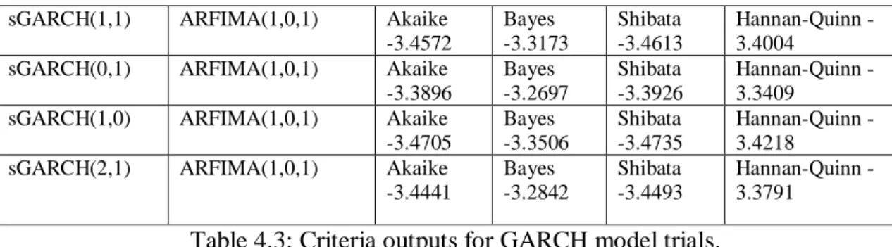
After determining our ARMA order now we should decide our GARCH order. GARCH(p,q) in which p is the order of the GARCH terms σ2 and q is the order of the ARCH terms ε2 . According to historical literature, GARCH (1,1) is mostly used and acknowledged as pretty enough order for most of the cases. Nevertheless, I have made some trials for order in RStudio and found the fittest order. I checked the results of (1,1), (0,1), (1,0), (2,1) and minimum Akaike criteria turned out to be order (1,0). RStudio output for GARCH order trials can be seen below.
20
sGARCH(1,1) ARFIMA(1,0,1) Akaike
-3.4572 Bayes -3.3173 Shibata -3.4613 HannanQuinn -3.4004
sGARCH(0,1) ARFIMA(1,0,1) Akaike
-3.3896 Bayes -3.2697 Shibata -3.3926 HannanQuinn -3.3409
sGARCH(1,0) ARFIMA(1,0,1) Akaike
-3.4705 Bayes -3.3506 Shibata -3.4735 HannanQuinn -3.4218
sGARCH(2,1) ARFIMA(1,0,1) Akaike
-3.4441 Bayes -3.2842 Shibata -3.4493 HannanQuinn -3.3791
Table 4.3: Criteria outputs for GARCH model trials.
So, the orders are determined as (1,1) for ARMA and (1,0) for GARCH. I combined these models and calculate GARCH terms for each period. Eventually, each type of our market activity and volatility variable is set and ready to be input of our final regression model. Let us remember our regression model again.
Market_Activityt =β0 +β1*Trend + β2*Market_Activityt-1 + β3*Volatilityt +
ε
tMy target is to set a strong model and find the relationship between volatility and market activity. As it is mentioned before there are 8 types of combinations, we should put all combinations of data into the model.
5. Empirical Results and Conclusion
I have taken model results for all combinations. A summary of results is as below:
ARMA(1,1)-GARCH(1,0)
Implied Volatility Actual Volatility ARMA(1,1)-GARCH(1,0) Actual Volatility ARMA(1,1)-GARCH(1,1) Option Trading Volume 0.9394** 2.6312* 1.1615 Option Open Interest 0.1837** 0.41 0.2119 Future Trading Volume 0.8903** 1.4363 2.5181
Future Open Interest 0.221** -0.3212 -0.2904
21 Coefficients are the regression models’ coefficients and it tells us the change in market activity when unit change in corresponding predictor. According to result tables, there is a strong positive relationship between implied volatility VSTOXX and market activity for derivatives. It doesn’t vary on activity or derivative types; it is always significant and positively linked. Conversely, actual volatility which is estimated by ARMA (1,1)-GARCH (1,0) model has only showed positive correlation with 5% significance for option trading volume. Just for curiosity and for the reason that it is the most used model in the literature I got results for GARCH (1,1) as well. Results slightly changed and 5% significance for option trading volume turned to insignificant. Even a change in model order affected significance. In literature studies vary for markets, models, model orders, time periods etc. So it is clear to understand why similar studies have different results. Both volatility types have different natures and it is very
acceptable to end up with different significance like my study denotes. Surprisingly, (Jeanneau and Micu 2003) finds very slightly different results for both volatility types, they were very similar overall. Yet, they have told that their results very surprising because of the fact that two types of volatility have not markedly different impact on market activity.
Another finding from the results is that derivative type has very weak effect on market activity. To make it clear, we observe same level of significance under the same volatility except the option trading volume under actual volatility. Our results are in line with many other researches. Numerous previous studies are inclined to find a positive relation between volatility and market activity. This is exactly what we have concluded for implied volatility. Also, as (Gökbulut et al. 2009) denoted, actual volatility has not showed significant relation with trading volume as my study has concluded. Shortly, many different studies share similar conclusions with this study and many not.
Previously applied methods are used on a different market and time period. Hence, this study’s results differ so cannot reflect exactly same results with others.
22
6. Reference Page
Albulescu, C.T. & Goyeau, D. (2011), Financial volatility and derivatives products: a bidirectional relationship, Scientific Annals of the "Alexandru Ioan Cuza" University of Iasi, Economic Sciences Section, Special Number, 57-69.
Angelos Siopis, & Bhaumiky, M. Karanasosy &A. Kartsaklas., (2008), Derivatives trading and the volume-volatility link in the indian stock market. William Davidson Institute Working Paper Number, p 935.
Baklacı, H , Kasman, A . (2006). AN EMPIRICAL ANALYSIS OF TRADING VOLUME AND RETURN VOLATILITY RELATIONSHIP IN THE TURKISH STOCK MARKET . Ege Academic Review , 6 (2) , 115-125 . Retrieved from https://dergipark.org.tr/tr/pub/eab/issue/39839/472388
Bollerslev, T. (1986). Generalized autoregressive conditional heteroskedasticity. Journal of Econometrics, 31(3), 307–327. https://doi.org/10.1016/0304-4076(86)90063-1
Çağlayan, E. (2011). The Impact of Stock Index Futures on the Turkish Spot Market. Journal of Emerging Market Finance, 10(1), 73–91.
https://doi.org/10.1177/097265271101000103 .
Cimen, Aysegul, (2018). The Impact of Derivatives on the Volatility of Turkish Stock Market. International Journal of Economic and Administrative Studies. Available at SSRN: https://ssrn.com/abstract=3340904
Donaldson, R. G., & Kamstra, M. J. (2005). VOLATILITY FORECASTS, TRADING VOLUME, AND THE ARCH VERSUS OPTION-IMPLIED
VOLATILITY TRADE-OFF. Journal of Financial Research, 28(4), 519–538. https://doi.org/10.1111/j.1475-6803.2005.00137.x
Gökbulut, İ , Köseoğlu, S , Atakan, T . (2009). The effects of the stock index futures to the spot stock market: a study for the Istanbul Stock Exchange . İstanbul Üniversitesi İşletme Fakültesi Dergisi , 38 (1) , 84-100 . Retrieved from
https://dergipark.org.tr/tr/pub/iuisletme/issue/9247/115692
Jeanneau, Serge, and Marian Micu. "Volatility and derivatives turnover: a tenuous relationship." BIS Quarterly Review, 2003, pp. 57-66.
23 Kasman, A., & Kasman, S. (2008). The impact of futures trading on volatility of the underlying asset in the Turkish stock market. Physica A: Statistical Mechanics and Its Applications, 387(12), 2837–2845. https://doi.org/10.1016/j.physa.2008.01.084
Chesney, M., Crameri, R., & Mancini, L. (2015). Detecting abnormal trading activities in option markets. Journal of Empirical Finance, 33, 263–275.
https://doi.org/10.1016/j.jempfin.2015.03.008
Perlin, M. S., Mastella, M., Vancin, D., & Ramos, H. (2020, March). A GARCH Tutorial with R. https://www.msperlin.com/blog/post/2020-03-29-garch-tutorial-in-r/
Narasimhan, M. S., & Kalra, S. (2014). The Impact of Derivative Trading on the Liquidity of Stocks. Vikalpa: The Journal for Decision Makers, 39(3), 51–66.
https://doi.org/10.1177/0256090920140304
Pan, J., & Poteshman, A. (2004). The Information of Option Volume for Future Stock Prices. NBER Working Paper, 872–908. https://doi.org/10.3386/w10925
Robinson, G. (1994) The effects of futures trading on cash market volatility: evidence from the London Stock Exchange, Review of Futures Markets, 13(2), 107-130.
Weber, E. J., & University of Western Australia. Business School. Economics. (2008). A Short History of Derivative Security Markets. Reed Business Education.
Yilgor, A. G. (2016). The effect of futures contracts on the stock market volatility: Pressacademia, 5(3), 307.
24
7. Appendices
#end of day price data readdata<-read.csv("price -2008-2009.csv")
tail(data)
#convert data to timeseries type
E_07<-ts(data[1:152,2],frequency=12)
plot(E_07)
#check if GARCH is appropriate
Box.test(e_07, lag=10 , type="Ljung-Box")
#to satisfy stationarity conditions diff and log taken
e_07=diff(log(E_07))
plot(e_07,ylab="",xlab="")
#important lag check, it wont be used though. I use auto.arima() acf(e_07)
pacf(e_07)
#arma order trials to find the best model
ar1<-arima(e_07,c(1,0,0))
ar1
ar2<-arima(e_07,c(2,0,0))
ar2
arma11<-arima(e_07,c(1,0,1))
arma11
##install library of garch
install.packages("rugarch")
library(rugarch)
plot(e_07)
install.packages("forecast")
require(forecast)
auto.arima(e_07, trace=TRUE)
auto.arima(E_07, trace=TRUE) #garch order trials for e_10
g1
<-ugarchspec(variance.model=list(model="sGARCH",garchOrder=c(1,1)),mean. model=list(armaOrder=c(1,1)),distribution.model="std")
garch11_07=ugarchfit(g1,data=e_07)
garch11_07 g2
<-ugarchspec(variance.model=list(model="sGARCH",garchOrder=c(0,1)),mean. model=list(armaOrder=c(1,1)),distribution.model="std")
garch01_07=ugarchfit(g2,data=e_07)
garch01_07 g3
<-ugarchspec(variance.model=list(model="sGARCH",garchOrder=c(1,0)),mean. model=list(armaOrder=c(1,1)),distribution.model="std")
garch10_07=ugarchfit(g3,data=e_07)
garch10_07 g4
<-ugarchspec(variance.model=list(model="sGARCH",garchOrder=c(2,1)),mean. model=list(armaOrder=c(1,1)),distribution.model="std")
garch21_07=ugarchfit(g4,data=e_07)
garch21_07
#full model coefficients
garch10_07@fit$coef
garch10_07@fit$sigma
25
library('quantmod')
library('tseries')
## option trading volume
op_tr_vol<-read.csv('option_trading_volume -2007sonrası.csv',header=T,sep=';')
#op_tr_vol<-xts(op_tr_vol[,2],order.by=as.Date(op_tr_vol[,1])) colnames(op_tr_vol)<-'o_t_v'
op_tr_vol_data=ts(op_tr_vol[61:212,2])
auto.arima(op_tr_vol_data, trace=TRUE)
op_tr_vol_log=diff(log(op_tr_vol_data))
findfrequency(op_tr_vol_log)
plot(op_tr_vol_log_07,main='Option Trading Volume')
adf.test(op_tr_vol_data,alternative='stationary',k=1)
adf.test(op_tr_vol_log,alternative='stationary',k=1) ## option open interest
op_opint_vol<-read.csv('option_open_interest -2007sonrası.csv',header=T,sep=';')
#op_opint_vol<-xts(op_opint_vol[,2],order.by=as.Date(op_opint_vol[,1])) colnames(op_opint_vol)<-'o_oi_v'
op_opint_vol_data=ts(op_opint_vol[,2])
auto.arima(op_opint_vol_data, trace=TRUE)
op_opint_vol_log=diff(log(op_opint_vol[,2]))
findfrequency(op_opint_vol_data)
plot(op_opint_vol_data,main='Option Open Interest Volume')
plot(op_opint_vol_log,main='Option Open Interest Volume')
adf.test(op_opint_vol_data,alternative='stationary',k=1)
adf.test(op_opint_vol_log,alternative='stationary',k=1) ## future trading volume
ft_tr_vol<-read.csv('future_traded_volume -2007sonrası.csv',header=T,sep=';')
#ft_tr_vol<-xts(ft_tr_vol[,2],order.by=as.Date(ft_tr_vol[,1])) colnames(ft_tr_vol)<-'f_t_v'
ft_tr_vol_data=ts(ft_tr_vol[,2])
auto.arima(ft_tr_vol_data, trace=TRUE)
ft_tr_vol_log=diff(log(ft_tr_vol[,2]))
findfrequency(ft_tr_vol_data)
plot(ft_tr_vol_data,main='Future Trading Volume')
plot(ft_tr_vol_log,main='Future Trading Volume')
adf.test(ft_tr_vol_data,alternative='stationary',k=1)
adf.test(ft_tr_vol_log,alternative='stationary',k=1) ## future open interest volume
ft_oi_vol<-read.csv('future_open_interest -2007sonrası.csv',header=T,sep=';')
#ft_oi_vol<-xts(ft_oi_vol[,2],order.by=as.Date(ft_oi_vol[,1])) colnames(ft_oi_vol)<-'f_oi_v'
ft_oi_vol_data=ft_oi_vol[,2]
auto.arima(ft_oi_vol_data, trace=TRUE)
ft_oi_vol_log=diff(log(ft_oi_vol[,2]))
findfrequency(ft_oi_vol_data)
plot(ft_oi_vol_data,main='Future Open Interest Volume')
plot(ft_oi_vol_log,main='Future Open Interest Volume')
adf.test(ft_oi_vol_data,alternative='stationary',k=1)
adf.test(ft_oi_vol_log,alternative='stationary',k=1) ##cox-stuart test for trend
op_tr_vol2<-read.csv('option_trading_volume -2007sonrası.csv',header=T,sep=';')
26
op_opint_vol2<-read.csv('option_open_interest -2007sonrası.csv',header=T,sep=';')
ft_tr_vol2<-read.csv('future_traded_volume -2007sonrası.csv',header=T,sep=';')
ft_oi_vol2<-read.csv('future_open_interest -2007sonrası.csv',header=T,sep=';')
## trend of the volume not mentioned in the thesis
install.packages("trend") library(trend) cs.test(op_tr_vol2[61:212,2]) cs.test(op_tr_vol_log) cs.test(op_opint_vol2[,2]) cs.test(op_opint_vol_log) cs.test(ft_tr_vol2[,2]) cs.test(ft_tr_vol_log) cs.test(ft_oi_vol2[,2]) cs.test(ft_oi_vol_log) install.packages("modifiedmk") library(modifiedmk) mkttest(op_tr_vol2[,2]) mkttest(op_opint_vol2[,2]) mkttest(ft_tr_vol2[,2]) mkttest(ft_oi_vol2[,2])
# implied volatility vstoxx stationarity test
vstoxx<-read.csv("vstoxx -2007 sonrası.csv",sep=";")
head(vstoxx)
plot(vstoxx[,2])
vst<-ts(vstoxx[,2],frequency=12)
vstoxx_log=diff((log(vst)))
cs.test(vstoxx[,2])
adf.test(vstoxx[,2],alternative='stationary',k=1)
cs.test(vstoxx_log)
adf.test(vstoxx_log,alternative='stationary',k=1)
##All combinations of derivatives-volatility-marketactivity tested in Lineer regressin
reg_vstoxx<-read.csv("regressiona_girecek_vstoxx -2007sonrası.csv",sep=";")
reg_vstoxx_07=reg_vstoxx[59:210,]
attach(reg_vstoxx_07)
findfrequency(OPT_TRADED_VOLUME)
Trend=seq_along(OPT_TRADED_VOLUME)
model_fit=lm(OPT_TRADED_VOLUME~Trend+OPT_TRADED_VOLUME_LAG+vstoxx_log,
data=reg_vstoxx_07)
summary(model_fit)
model_fit$model
reg_vstoxx<-read.csv("regressiona_girecek_vstoxx -2007sonrası.csv",sep=";")
reg_vstoxx_07=reg_vstoxx[59:210,]
attach(reg_vstoxx_07)
findfrequency(OPT_OPEN_INTEREST)
Trend=seq_along(OPT_OPEN_INTEREST)
model_fit=lm(OPT_OPEN_INTEREST~Trend+OPT_OPEN_INTEREST_LAG+vstoxx_log,
data=reg_vstoxx_07)
summary(model_fit)
model_fit$model
findfrequency(FUT_TRADED_VOLUME)
27
model_fit=lm(FUT_TRADED_VOLUME~Trend+FUT_TRADED_VOLUME_LAG+vstoxx_log,
data=reg_vstoxx_07)
summary(model_fit)
model_fit$model
findfrequency(FUT_OPEN_INTEREST)
Trend=seq_along(FUT_OPEN_INTEREST)
model_fit=lm(FUT_OPEN_INTEREST~Trend+FUT_OPEN_INTEREST_LAG+vstoxx_log,
data=reg_vstoxx_07)
summary(model_fit)
model_fit$model
---# insert actual volatility 2008-2009 into model after without diff
reg_garch<-read.csv("regressiona_girecek_garch -2007sonrası.csv",sep=";")
#reg_garch_07=reg_garch[59:210,] attach(reg_garch)
findfrequency(OPT_TRADED_VOLUME)
Trend=seq_along(OPT_TRADED_VOLUME)
model_fit=lm(OPT_TRADED_VOLUME~Trend+OPT_TRADED_VOLUME_LAG+garch10,dat a=reg_garch)
summary(model_fit)
model_fit$model
findfrequency(OPT_OPEN_INTEREST)
Trend=seq_along(OPT_OPEN_INTEREST)
model_fit=lm(OPT_OPEN_INTEREST~Trend+OPT_OPEN_INTEREST_LAG+garch10,dat a=reg_garch)
summary(model_fit)
model_fit$model
findfrequency(FUT_TRADED_VOLUME)
Trend=seq_along(FUT_TRADED_VOLUME)
model_fit=lm(FUT_TRADED_VOLUME~Trend+FUT_TRADED_VOLUME_LAG+garch10,dat a=reg_garch)
summary(model_fit)
model_fit$model
findfrequency(FUT_OPEN_INTEREST)
Trend=seq_along(FUT_OPEN_INTEREST)
model_fit=lm(FUT_OPEN_INTEREST~Trend+FUT_OPEN_INTEREST_LAG+garch10,dat a=reg_garch) summary(model_fit) model_fit$model