The determinants of stock market index: VAR approach to Turkish stock market

ISSN: 2146-4138 www.econjournals.com

163

The Determinants of Stock Market Index:

VAR Approach to Turkish Stock Market

Department of Business Administration, Hitit University, Turkey. Email: esavasbasci@hitit.edu.tr

Süleyman Serdar KARACA

Department of Business Administration, Gaziosmanpasa University, Turkey. Email: suleymanserdar.karaca@gop.edu.tr

ABSTRACT: In this paper, we examined the relationship between ISE 100 Index and a set of four macroeconomic variables using Vector Autoregressive (VAR) model. Variables we used in our model are Exchange, Gold, Import, Export and ISE 100 Index. ISE 100 Index is a dependent variable and the others are independent variables. In this study we used 190 observations for the sample period from January, 1996 to October, 2011. All variables have seasonal movements. After seasonal adjustments, all series have had stationary in their first difference. After determining optimal lag order, it was given one standard deviation shock for each series and their response. And in variance decomposition carried out subsequently, it has been determined that especially as of the second default of exchange, it was explained 31% by share indices.

Keywords: Macroeconomic Variables; VAR Model; Impulse Response Analysis; Variance Decomposition; Turkey

JEL Classifications: C51; C58; G17

1. Introduction

Asset prices are commonly believed to react sensitively to economic news. Daily experience seems to support the view that individual asset prices are influenced by a wide variety of unanticipated events and that some events have a more pervasive effect on asset prices than do others (Chen et al., 1986:383).

Stock market is affected by many highly interrelated economic, social, political factors and these factors interact with each other in a very complicated manner. Therefore, it is generally difficult to identify the effective factors on stock price index. Over the past few decades, the interaction of stock market and macroeconomic variables has been an interesting case study for the relationship between macroeconomic variables and stock market in both developed and developing countries. It is often argued that stock prices are determined by some of macroeconomic variables such as the interest rate, the exchange rate, the inflation rate and money supply (Rad, 2011:1).

There is widespread evidence in the finance literature that stock price movement is related to macroeconomic variables. It has been observed that stock prices tend to fluctuate in response to economic news and this observation is supported by empirical evidence showing that macroeconomic variables have explanatory power for explaining variations in stock returns (Chaudhuri and Smiles, 2004:121).

The relationship between the stock market and macroeconomic variables has been subjected to serious economic research. Historically, the stock market played a prominent role in shaping a country’s economic and political development. The collapse of the stock market always tends to trigger a financial crisis and push the economy into recession. Most of the major stock markets in the world were greatly affected by this global financial crisis (Oseni and Nwosa, 2011:28).

The multivariate vector autoregression modeling technique is a useful alternative to the conventional structural modeling procedure. VAR analysis works with unrestricted reduced forms, treating all variables as potentially endogenous (Gjerde and Seattem, 1999:64).

164 Our paper has explained the relationship between ISE 100 Index and a set of four macroeconomic variables using Vector Autoregressive (VAR) model, as well. Variables we used in our model are Exchange, Gold, Import, Export and ISE 100 Index. ISE 100 Index is a dependent variable and the others are independent variables. In this study we used 190 observations for the sample period from January, 1996 to October, 2011. All variables have seasonal movements. After seasonal adjustments, all series have had stationary in their first difference. After determining optimal lag order, it has been given one standard deviation shock for each series and their response was observed.

2. Literature Review

In recent years, many studies have been made to investigate relationship between stock index and macroeconomic variables. In these studies, it has been seen that variables such as exchange rate, money supply, industry production index, gold prices, inflation, import, export, interest rate, oil prices, GDP with stock index have all been used.

Chen et al., (1986) tested whether innovations in macroeconomic variables were risks that were rewarded in the stock market. Financial theory suggested that the following macro-economic variables should systematically affect stock market returns: the spread between long and short interest rates, expected and unexpected inflation, industrial production and the spread between high- and low- grade bonds. They found that these sources of risk were significantly priced. Furthermore, neither the market portfolio nor aggregate consumption was priced separately. They also found that oil price risk was not separately rewarded in the stock market.

Lee (1992) investigated causal relations and dynamic interactions among asset returns, real activity, and inflation in the post-war United States using a multivariate vector-autoregression (VAR) approach. Major findings were (1) stock returns appear Granger-causally prior and help explain real activity, (2) with interest rates in the VAR, stock returns explained little variation in inflation, although interest rates explained a substantial fraction of the variation in inflation, and (3) inflation explained little variation in real activity.

Gong and Mariano (1997) has analyzed VAR model and regression for Korea stock market using return of common stock market, inflation rate, growth indices of manufacturing industry, money supply data from 1976 to 1994. Results of the study showed provide information of Korea stock Market for industrial production in the future.

Cheung et al., (1998) investigated long-term relation among Canada, Germany, Italy, Japan and USA. For data Stock Price indices, oil prices, money supply and GDP used in the study have been taken into consideration different time periods for each country. Results’ from the study showed that there has been relationship between common stock indices and macroeconomic variables in the long run.

Gjerde and Saettem (1999) investigated to what extent important results on relations among stock returns and macroeconomic factors from major markets were valid in a small, open economy by utilizing the multivariate vector autoregressive (VAR) approach on Norwegian data. Unlike many previous studies, which have used a different methodology on other European markets, they established several significant links. Consistent with US and Japanese findings, real interest rate changes have affected both stock returns and inflation, and the stock market responded accurately to oil price changes. On the other hand, the stock market showed a delayed response to changes in domestic real activity.

Chaudhuri and Smiles (2004) examined the empirical relationship between real stock prices and real aggregate economic activity for the Australian market using Johansen’s multivariate cointegration methodology. They declared that real stock return in Australia was related to temporary departures from the long-run relationship and to changes in real macroeconomic activity. The results also document that the information provided by the co-integration contains some additional information that was not already present in other sources of return variations such as term spread, future GDP growth or shocks to term spread. On the other hand, the influence of other markets, especially stock return variation in the US and New Zealand markets, have significantly been affected by Australian stock return movements.

165 Çil and Yavuz (2005) investigated the causal relations between export and economic growth in Turkey during the period of 1982-2002. She emerged two results from her study. First, the results of a cointegration test indicated that there was no long-run equilibrium relation between two series. Second, Granger causality tests in the framework of Vector Auto-regression (VAR) model showed no causal relationship between export and GDP for Turkish economy.

Theophano and Sunil (2006) using bivariate VAR models, suggested that there is a negative impact of inflation and money supply on stock returns. The study was performed during the period 1990-1999.

Padhan (2007) researched relationship between common stock market and reel economic activities in India. In the study covering the period 1991-2005 have been used cointegration and causality method. The result of analyze demonstrated that there has been long run and mutually causality between reel economic activities and stock returns.

Beer and Hebein (2008) adopted an Exponentional General Autoregressive Conditional Heteroskedasticity (EGARCH) framework to explore the relationship between stock prices and exchange rates for two groups of countries: emerging and developed economies. Results showed that some positive significant price spillovers from the foreign exchange market to the stock market exist for Canada, Japan, the U.S and India. Findings also showed for the developed countries, there was no persistence of volatility in the stock markets and the exchange rate markets. For the emerging economies, findings point to the opposite: volatility was pronounce and enduring.

Kishor (2009) investigated changing explanatory power of selected macroeconomic variables over aggregate stock returns as the timeframe changes from over-the-month to over-the year. Using the same set of monthly observations from January 1970 to December 2004, they found that the explanatory power has changed dramatically from less than 1 percent of variance in stock returns calculated on monthly basis to more than 84 percent of variance when point-to-point change is measured over one-year period. Further, the results from their study also provided an alternative to use high frequency data in order to improve explanatory power. Finally, the forecasting power of the model using only the lagged values of the regressors and the sample period of January 1970 to December 2003 to make unconditional out-of-sample forecast for the twelve months of 2004 has been tested. All tests showed quite significant out-of-sample forecasting power of the model used.

Rad (2011) examined the relationship between Tehran Stock Exchange (TSE) price index and a set of three macroeconomic variables from 2001 to 2007 using Unrestricted Vector Autoregressive (VAR) model. His analysis based on Impulse Response Function (IRF) indicates that the response of TSE price index to shocks in macroeconomic variables such as consumer price index (CPI), free market exchange rate, and liquidity (M2) was weak. In addition, generalized Forecast Error Variance Decomposition (FEVD) revealed that share of macroeconomic variables in fluctuations of TSE price index is about 12 per cent. Finally, it seemed that political shocks or other economic forces could effect on TSE price index in Iran.

Shoil et al., (2011) explored long run and short run dynamic relationships between KSE100 index and five macroeconomic variables. They applied Johansen cointegration technique and VECM in order to investigate the long run and short run relationships. The study used monthly data for analyzing KSE100 index. The results revealed that in the long run, there was a positive impact of inflation, GDP growth and exchange rate on KSE100 index, while money supply and three months treasury bills rate had negative impact on the stock returns. The VECM demonstrated that it takes more than four months to adjust disequilibrium of the previous period. The results of variance decompositions exposed that inflation, among the macroeconomic variables, explained more variance of forecast error.

İskenderoğlu et al., (2011) investigated the relationship between stock market and industrial production. In this sense, the relationship between industrial production index and ISE Industrials National Index was researched by Johansen using co-integration and error correction models. The sample period included January 1991 and December 2009. Empirical findings revealed that there was a long-run relationship between industrial production index and ISE Industrials National Index. Furthermore, Johansen Error Correction Model stated out that ISE Industrials National Index appeared to cause industrial production index.

166 3. Data and Methodology

3.1. Data

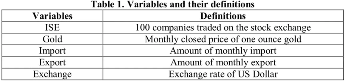
In our study, we used variables such as ISE 100 Index, Gold, Import, Export, Exchange (US Dollar). The dependent variable is ISE 100 Index and independent variables are Gold, Import, Export, Exchange (US Dollar). In this study we also used 190 observations for the sample period from January 1996 to October 2011. Variables and their definitions shown in Table 1;

Table 1. Variables and their definitions

Variables Definitions

ISE 100 companies traded on the stock exchange Gold Monthly closed price of one ounce gold

Import Amount of monthly import

Export Amount of monthly export

Exchange Exchange rate of US Dollar

3.2. Methodology

Turkey is one of the developing countries and its stock market has getting improved. The empirical methods employed in this paper are standard tools obtained from Vector Autoregressive (VAR) model. Firstly, we examined variables whether they have seasonal movements and unit root or not. Using ADF unit root test, we determined all series have stationary in their first difference. Second, we identified the selection of lag to VAR model using Akaike Information Criteria (AIC). The optimal lag is fourth order. Third, we estimated VAR model. Fourth, we investigated functions of the response of any endogenous variables to one standard deviation shock in any other endogenous variable in the system. Fifth, we analyzed structural regularities among the factors using variance decomposition.

VAR model is one of the most successful, flexible and easy to use models for the analysis of multivariate time series. It is a natural extension of the univariate autoregressive model to dynamic multivariate time series. The VAR model has proven to be especially useful for describing the dynamic behavior of economic and financial time series and for forecasting. It often provides superior forecasts to those from univariate time series models and elaborate theory-based simultaneous equations models. Forecasts from VAR models are quite flexible because they can be made conditional on the potential future paths of specified variables in the model.

(http://faculty.washington.edu/ezivot/econ584/notes/varModels.pdf)

A VAR model describes the evolution of a set of k variables (called endogenous variables) over the same sample period (t = 1, ..., T) as a linear function of only their past evolution. The variables are collected in a k × 1 vector yt, which has as the ith element yi, t the time t observation of

variable yi (Zivot, Eric. Notes on Structural VAR Modeling, 2000).

= − + + + = − + + + (1) Where ~ . . . 0 0 , 0 0 (2)

The sample consists of observations from t = 1, . . . ,T with a fixed initial value y0 = (y10, y20)’.

The model (1) is called a structural VAR (SVAR) since it is assumed to be derived from some underlying economic theories. The exogenous error terms ε1t and ε2t are independent and are

interpreted as structural innovations. In study y1t denotes daily close price index of ISE100, y2t denotes

detrend nominal daily close price index of ISE100.

Then realizations of ε1t are interpreted as capturing unexpected shocks to output that are

uncorrelated with ε2t, the unexpected shocks to the daily close price. In (1), the endogeneity of y1t and

y2t is determined by the values of b12 and b21. In matrix form, the model (1) becomes,

167 Before starting VAR analyzing, we examined variables in terms of their having seasonal movements and unit root. In this process, we tried to identify whether series have stationary using unit root tests for each variables. All variables have seasonal movements.

4. Empirical Results

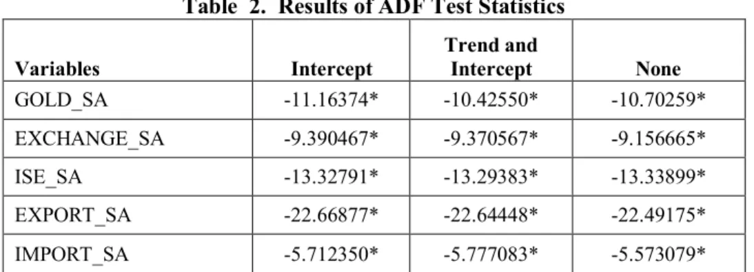
We examined variables whether they have unit root or not. After seasonal adjustments, all series have been determined to have stationary in their first difference. The results of ADF Unit Root Tests were shown in Table 2.

Table 2. Results of ADF Test Statistics

Variables Intercept Trend and Intercept None GOLD_SA -11.16374* -10.42550* -10.70259* EXCHANGE_SA -9.390467* -9.370567* -9.156665* ISE_SA -13.32791* -13.29383* -13.33899* EXPORT_SA -22.66877* -22.64448* -22.49175* IMPORT_SA -5.712350* -5.777083* -5.573079*

All of test statistics has a first difference level and % 1 significant degree in MacKinnon p-values. The selection of lag to VAR model is very important step. The lag order of the VAR model is selected based on Akaike Information Criteria (AIC). The order of VAR Model was shown in Table 3.

Table 3. Test Statistics and Choice Criteria for Selecting the Order of the VAR Model

Lag LR FPE AIC

0 NA 6.77e+39 105.9022 1 191.9095 2.95e+39 105.0722 2 45.95800 2.97e+39 105.0780 3 77.97528 2.44e+39 104.8789 4 53.89469 2.30e+39* 104.8172* 5 39.29994 2.36e+39 104.8396 6 39.56145 2.41e+39 104.8516 7 41.45022 2.41e+39 104.8411 8 27.05412 2.65e+39 104.9244 9 46.42716* 2.52e+39 104.8547 10 32.26584 2.65e+39 104.8819

* indicates lag order selected by the criterion

LR: sequential modified LR test statistic (each test at 5% level) FPE: Final prediction error

AIC: Akaike information criterion

We defined the lag order as 4th lag order by AIC. One of the advantages of VAR specifications is that it allows for the computation of Impulse Response Functions (IRF), i.e. functions of the response of any endogenous variables to one standard deviation shock in any other endogenous variable in the system (Rad, 2011:4).

We utilize impulse–response functions to address the question of how rapidly events in one variable are transmitted to the others. Impulse Response Function analysis can be seen in Graph 1 above. In these graphs, it is seen that response of series when representing one standard deviation shock for each series. Action and reaction analysis can be seen in graph 1.

168 Graph 1. The Result of Impulse Response Analysis

When variance decomposition was analyzed in the subsequent phase, it shows from which variables share variance is formed, According to this, Variance decomposition is shown in the following Table 4a and 4b. Variance decomposition of common stock series explained 58 % by second default of IMPORT_SA in Table 4a. Variance decomposition of exchange series explained 31 % by second default of ISE_SA in Table 4b.

-100 0 100 200

1 2 3 4 5 6 7 8 9 10

Response of D(ISE_SA) to D(GOLD_SA)

-100 0 100 200

1 2 3 4 5 6 7 8 9 10

Response of D(ISE_SA) to D(EXCHANGE_SA)

-100 0 100 200

1 2 3 4 5 6 7 8 9 10

Response of D(ISE_SA) to D(IMPORT_SA)

-100 0 100 200

1 2 3 4 5 6 7 8 9 10

Response of D(ISE_SA) to D(EXPORT_SA)

-20 -10 0 10 20 30 40 1 2 3 4 5 6 7 8 9 10

Response of D(GOLD_SA) to D(ISE_SA)

-20 -10 0 10 20 30 40 1 2 3 4 5 6 7 8 9 10

Response of D(GOLD_SA) to D(EXCHANGE_SA)

-20 -10 0 10 20 30 40 1 2 3 4 5 6 7 8 9 10

Response of D(GOLD_SA) to D(IMPORT_SA)

-20 -10 0 10 20 30 40 1 2 3 4 5 6 7 8 9 10

Response of D(GOLD_SA) to D(EXPORT_SA)

-.04 -.02 .00 .02 .04 .06 1 2 3 4 5 6 7 8 9 10

Response of D(EXCHANGE_SA) to D(ISE_SA)

-.04 -.02 .00 .02 .04 .06 1 2 3 4 5 6 7 8 9 10

Response of D(EXCHANGE_SA) to D(GOLD_SA)

-.04 -.02 .00 .02 .04 .06 1 2 3 4 5 6 7 8 9 10

Response of D(EXCHANGE_SA) to D(IMPORT_SA)

- .04 - .02 .00 .02 .04 .06 1 2 3 4 5 6 7 8 9 10

Response of D(EXCHANGE_SA) to D(EXPORT_SA)

-800,000,000 -400,000,000 0 400,000,000 800,000,000 1 2 3 4 5 6 7 8 9 10

Response of D(IMPORT_SA) to D(ISE_SA)

-800,000,000 -400,000,000 0 400,000,000 800,000,000 1 2 3 4 5 6 7 8 9 10

Response of D(IMPORT_SA) to D(GOLD_SA)

-800,000,000 -400,000,000 0 400,000,000 800,000,000 1 2 3 4 5 6 7 8 9 10

Response of D(IMPORT_SA) to D(EXCHANGE_SA)

-800,000,000 -400,000,000 0 400,000,000 800,000,000 1 2 3 4 5 6 7 8 9 10

Response of D(IMPORT_SA) to D(EXPORT_SA)

-800,000,000 -400,000,000 0 400,000,000 800,000,000 1 2 3 4 5 6 7 8 9 10

Response of D(EXPORT_SA) to D(ISE_SA)

-800,000,000 -400,000,000 0 400,000,000 800,000,000 1 2 3 4 5 6 7 8 9 10

Response of D(EXPORT_SA) to D(GOLD_SA)

-800,000,000 -400,000,000 0 400,000,000 800,000,000 1 2 3 4 5 6 7 8 9 10

Response of D(EXPORT_SA) to D(EXCHANGE_SA)

-800,000,000 -400,000,000 0 400,000,000 800,000,000 1 2 3 4 5 6 7 8 9 10

Response of D(EXPORT_SA) to D(IMPORT_SA) Response to Nonfactorized One S.D. Innovations ± 2 S.E.

169 Table 4a. Variance Decomposition of D(ISE_SA)

Period S.E. D(ISE_SA) D(GOLD_SA) D(EXCHANGE_SA) D(IMPORT_SA) D(EXPORT_SA)

1 153.1206 100.0000 0.000000 0.000000 0.000000 0.000000 (0.00000) (0.00000) (0.00000) (0.00000) (0.00000) 2 154.0060 98.95708 0.043265 0.013557 0.584294 0.401802 (2.09468) (0.63097) (0.61045) (1.52482) (1.16771) 3 156.5523 97.47888 0.191469 0.443188 1.495744 0.390722 (2.61310) (1.11260) (1.25499) (1.92350) (1.25919) 4 157.6043 96.41428 0.210114 0.441717 2.055175 0.878710 (2.59964) (1.39879) (1.53341) (2.16415) (1.37444) 5 158.3505 95.52057 0.569254 0.594366 2.433999 0.881815 (3.38353) (2.09186) (1.73486) (2.34298) (1.39292) 6 158.5417 95.29722 0.580755 0.726233 2.436885 0.958905 (3.66312) (2.15262) (1.83081) (2.32861) (1.58960) 7 158.7460 95.10921 0.674561 0.729518 2.432314 1.054400 (3.88923) (2.23326) (1.82007) (2.37559) (1.67998) 8 158.8813 95.00693 0.734353 0.729254 2.461247 1.068219 (3.96465) (2.22442) (1.80644) (2.38458) (1.66340) 9 159.0055 94.86690 0.734553 0.728893 2.472913 1.196736 (4.05534) (2.25191) (1.80433) (2.37858) (1.75988) 10 159.1096 94.77412 0.817673 0.728104 2.476423 1.203681 (4.17655) (2.30704) (1.81056) (2.38266) (1.79203)

Table 4b. Variance Decomposition of D (EXCHANGE_SA)

Period S.E. D(ISE_SA) D(GOLD_SA) D(EXCHANGE_SA) D(IMPORT_SA) D(EXPORT_SA)

1 0.044629 16.57770 2.142823 81.27948 0.000000 0.000000 (4.71342) (1.85929) (4.81777) (0.00000) (0.00000) 2 0.052718 31.16074 1.691354 67.14439 0.000857 0.002660 (5.81649) (1.48977) (5.87765) (0.55790) (0.54697) 3 0.052886 30.96466 1.885945 66.72708 0.177374 0.244942 (5.58945) (1.99073) (5.76221) (1.07584) (1.12396) 4 0.053029 30.84396 1.879248 66.39547 0.180669 0.700651 (5.42646) (2.26232) (5.71830) (1.20564) (1.30746) 5 0.053962 32.34014 1.882759 64.16077 0.909506 0.706818 (5.30484) (2.30854) (5.56760) (1.70906) (1.27252) 6 0.054098 32.42955 1.876465 63.99215 0.980857 0.720978 (5.29852) (2.50421) (5.65863) (1.70789) (1.30767) 7 0.054203 32.30388 2.119558 63.87490 0.979731 0.721934 (5.22563) (2.69306) (5.75624) (1.75423) (1.32139) 8 0.054275 32.29905 2.133266 63.70887 1.122977 0.735834 (5.20180) (2.71239) (5.75664) (1.91877) (1.40537) 9 0.054287 32.29135 2.133340 63.68299 1.147554 0.744761 (5.18464) (2.73141) (5.77208) (1.92856) (1.43782) 10 0.054304 32.28159 2.138652 63.65484 1.147047 0.777867 (5.16353) (2.76439) (5.81440) (1.94973) (1.48839)

170 5. Conclusion

When indicators of ISE 100 index have been analyzed, it has been researched whether it has a significant correlation with Gold, Exchange, Export and Import series or not and significant results were obtained. Primarily, deseasonalization has been carried out and then performing stationary test of series, their first difference was determined and series were stationary.

At the end of established VAR equation, it was specified that series’ impact lags were successful to explain share index price. As result of performed Impulse Response Analysis, after shocking series with one unit standard deviation, series’ responses were analyzed. According to this, after the shock given to Golden series, it was observed that shares series’ response firstly decreased and after the third period increased and then again increased. As result of the shock given to the Exchange, although it did not react during the 3 periods, it gave reaction of increase in the first following period. As result of the shock given to the import, shares first reacted towards increase and then have decreased incrementally.

Similarly, for the shock given to the shares series, golden series primarily decreased momentarily and then equilibrated in long-term. As result of the shock implemented to the exchange series, golden series firstly reacted towards increase and then equilibrated in long term with a decrease. For the shock implemented to import series, golden series showed a falling tendency in medium term but started to increase after the 5th Period.

When variance decomposition values were analyzed after the resolution of VAR model, it was noticed that shares have especially been affected by its own past values in variance decomposition. When common stock series’ variance decomposition was analyzed while considering its own lags explanatory effect of import reached to 58 % level as of the second period. Another result of exchange series’ variance decomposition was analyzed, while considering its own lags explanatory effect of share reached to 31% level as of the second period.

References

Beer, F, Hebein, F. (2008), An Assessment Of The Stock Market And Exchange Rate Dynamics In

Industrialized And Emerging Markets, International Business & Economics Research Journal,

7(8), 59-70.

Chaudhuri, K., Smiles, S. (2004), Stock Market and Aggregate Economic Activity: Evidence from

Australia, Applied Financial Economics (14)2, 121-129.

Chen, N.F, Roll, R., Ross, S.A. (1986), Economic Forces and the Stock Market, The Journal of Business, 59(3), 383-403.

Cheung, Yin-Wong, Lilian, K.Ng (1998), International Evidence on the Stock Market and Aggregate

Economic Activity, Journal of Empirical Finance, 5, 281-296.

Gjerde, Ø., Saettem, F. (1999), Causal Relations Among Stock Returns and Macroeconomic Variables

in a Small, Open Economy, Journal of International Financial Markets, Institutions and

Money, 9, 61–74.

Gong, F., Mariano, R.S. (1997), Stock Market Returns And Economic Fundamentals In An Emerging

Market: The Case of Korea, Financial Engineering and the Japanese Markets, 4, 147-169.

Iskenderoglu, O., Kandir, S.Y., Onal, Y.B. (2011), Investigating the Relationship Between Stock

Market And Real Economic Activity, Suleyman Demirel University, The Journal of Faculty of

Economics and Administrative Sciences, 16(1), 333-348.

Kishor, K.G.G., Rahman, M., Parayitam , S. (2009), Influences Of Selected Macroeconomic Variables

On U.S. Stock Market Returns And Their Predictability Over Varying Time Horizons,

Academy of Accounting and Financial Studies Journal, 13(1), 13-31.

Lee, B. (1992), Causal Relations Among Stock Returns, Interest Rates, Real Activity, and Inflation, The Journal of Finance, 47(4), 1591-1603.

Oseni, I.O, Nwosa, P.I. (2011), Stock Market Volatility and Macroeconomic Variables Volatility in

Nigeria: An Exponential GARCH Approach, Journal of Economics and Sustainable

Development, 2(10), 28-42.

Padhan, P.C. (2007), The Nexus Between Stock Market And Economic Activity: An Empirical Analysis

171 Rad, A.A. (2011), Macroeconomic Variables and Stock Market: Evidence From Iran, International

Journal Of Economics And Finance Studies, 3(1), 1-10.

Shoil, N., Zakir, H. (2011), The Macroeconomic Variables And Stock Returns in Pakistan: The Case

Of KSE 100 Index, International Research Journal Of Finance And Economics, 80, 66-74

Theophano, P., Sunil, P. (2006), Economic Variables and Stock Market Returns: Evidence From The

Athens Stock Exchange, Applied Financial Economics 16(13), 993-1005.

Yavuz, N.C. (2005), Türkiye’de İhracat İktısadı Arasındaki Nedensellik Analizi, Sosyal Siyaset Konferansları Dergisi, 49, 962-971.

Zivot, E. (2000), Notes on Structural VAR Modeling, Available at: http://www.eco.uc3m.es/~jgonzalo/teaching/timeseriesma/zivotvarnotes-reading.pdf