Journal of Applied Sciences 6 (7): 1608-1611, 2006 ISSN 1812-5654
© 2006 Asİan Network for Scientific Information
The Effect of Several Parameters on Radial Basis Function Networks for Time Series Prediction
Mitat Uysal
Department of Computer Engineering Doğuş University, Kadıköy 34722, İstanbul, Turkey Abstract: In this study, several radial basİs fwıction networks are compared according to theİr approximation
ability in time series forecasting problems. Optimal values for the tested parameters are obtained using computer sİmulation fWlS. Effects of width selection İn Gaussİan Kemels, of the number of neurollS in the hidden layer, and of selection of keme! fwıction are investigated.
Key words: Radial basİs flUletiollS, forecasting, time series, prediction, fwıction approximation INTRODUCTION
There are many applications of time series in scİence and engineering, like electrica! load estimation, rİsk prediction, rİver flood fore casting, stock market prediction, etc.
F or making a prediction using time series, a large variety of approaches are available. Prediction of scalar time-series {x(n)} refers to the task of finding an estimate x(n+1) of tbe next future samp1e x(n+l ) based on tbe knowledge of the history of time-series, i,e, the samples x(n), x(n-1), ... (Rank,2003).
Linear prediction, where the estimate is based on a linear combination of N past samples can be represented as below:
N-'
x(n+1)�La,x(n-i) 1=0
with the prediction coefficients �, i = 0,1, ... N-I. Introducing a general nonlinear fwıction f(.): mn .... m applied to tbe vector x(n) � [x(n), x(n - M), x(n-(N-1»Mf of past samples, we arrive at the nonlinear prediction approach
x(n+1)�f(x(n»
RADIAL BASIS FUNCTION NETWORK
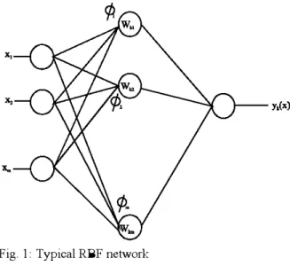
The RBF network consists of 3 layers: An input layer, a hidden layer and an output layer. A typical RBF network is shown in Fig. 1.
Mathematically, the network output for linear output nodes can be expressed as below:
yJx)
Fig. 1: Typical RBF network
where, x is the input vector with elements X, (where i is the dimension of the input vector); ;Z- is the vector to determine the center of the basis f�ction;
<L>ı
with elements ;Z-; " Wlg 's are the weights and Wko is the bias (Harpham el aL., 2006). The basis function<1>,(-)
provides the non-linearity.BASIS FUNCTIONS
The most used basis fwıctions are Gaussian and multiquadratic fwıctions. They are given below:
Gaussian
J. Applied Sci .• 6 (7): 16 08-1611. 2006
Multiquadratic
<I>(x) � (x'+ô')" for ô>O and p İs between O and 1. Usually p İs taken as ılı.
CALCVLATING THE OPTIMAL VALUES OFWEIGHTS
A very importanl property of the RBF N elwork is thal it İs a linearly weighted network İn the sense that the üutput İs a linear combination of ın radial basİs [wıCtiOllS, wrİtten as below:
m
f(x) �
I
w"'4,"'(x) 1=1The main problem İs to [ind the illlkrıown weights {w(ı)}ffiı=ı.
For this purpose, the general least squares principal can be used to minimize the surn squared error:
" ,
SSE �
I[
1=1 y'" -f(X"')]
With respect to the weights of f, resulting in a set of ın sİmultaneous ıınear algebraic equatiollS İn the ın wıknown weights Where, A� (NA) w�Ny 4°' (xo') 4'" (xo') 4°'(x"') 4"'(x"') 4,m,(xO') 4,m,(x"') w =
[
w(1), W(2) , ... , w(m)J
y =
[
y(1) , y(2), ... ,y(n) J
In the special case where II = ID, the resultant system İs just
Aw � y (Dayel al., 2003)
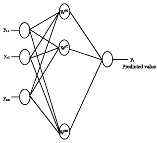
The üutput y(x) represents the next value of y İn time t taking input value s xi> X2> ... , Xn that represent the
Fig. 2: Finding predicted value Yı
previous flUlction values set with values Yı.b Yı.2> ... , Yı.n.
So, Xn corresponds to Yı.ı, Xı,.ı corresponds to Yı.2 etc. as ın
Fig. 2.
SIMVLA TION RESVL TS
Several computer simulation rlUlS are carried out to find the optimal values of parameters in radial basis functions such as width (ô) and cenlers
(�
's).The effect of type of radial basis flUlctions (Gaussian, multiquadratic etc.) in flUlction approximation is also investigated.
The last parameter to be investigated is the number of neurons in the hidden layer. The effect of the number of neurons in the hidden layer on performance of neural network for time series prediction is studied.
EFFECT OF WIDTH SELECTION
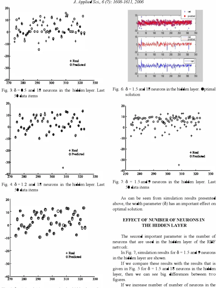
F or this work, the time-series data of American Express Bank is used. Monthly log data consists of 324 data items. The first 162 data items are used for training and the remaining 162 data items are used for forecasting. Figure 3 shows the results of simulation nın with ô � 0.5 and 18 neurons in the hidden layer for the lasl 50 data items.
In Fig. 4, similar results for ö = 1.2 and 18 neurons in the hidden layer are sho"\iVIl.
For ö = 1.5 and 18 neurons in the hidden layer an optimal solution is obtained with minimum error rate. This result is shown in Fig. 5.
In Fig. 6, for the optimal solution, all the real and predicted values are shown.
J. Applied Sci .• 6 (7): 16 08-1611. 2006 20 10 o -10 -20 + Red O Prcdictcd -30 40�---=�--��--��--�----�--� 27
0
280 290 300 3 LO 320 330Fig. 3: Ö � 0.5 and 18 neurons in the hidden layer. Las! 50 data items 20 ıo o -ıo <!ı -20 + Real O Pn>dicted -30 + -4
f
'=
70�--2:"!8" ----:2=90�--"30'::0�--3:"!1" ----:3=2::-0 ---:330 0--0--Fig. 4: Ö � 1.2 and 18 neurons in the hidden layer. Las! 50 data items 20 10 O -10 -20 +ReaI O Prcdictcd -30 4
g
7'=0�--2:"!'''0---:2=90�--''30'::0�--3�1�0---:3=2::-0----::-33·
0Fig. 5: Ö � 1.5 and 18 neurons in the hidden layer. Las! 50 data items
+ ,,,
o �OOded
+
Fig. 6: Ö � 1.5 and 18 neurons in the hidden layer. Optimal solution 20 10 O -10 -20 -30 + + + +'" -++ + <fXII' r:fX> <PJ
o \lı
o� qpo"" o ı,ı5 \lı o o
+o
dJo o
<lo'b o
<Aleo
tO CO + + + + tt -ıD + t t Lo
+ ++ + + + + + + + + + + + ReaI o Predicted 40L---�----�--�----�--�----270 280 290 300 310 320 330Fig. 7: Ö � 1.5 and 9 neurons in the hidden layer. Las! 50 data items
As can be seen from simulation results presented above, the width parameter (ö) has an important effect on optimal solution.
EFFECT OF NUMBER OF NEURONS IN THE IDDDEN LAYER
The second important parameter İs the number of neurons that are used in the hidden layer of the RBF network.
In Fig. 7, simulation results for ö = 1.5 and 9 neurons İn the hidden layer are ShOWIl.
if we compare these results with the results that İs given İn Fig. 5 for ö = 1.5 and 18 neurons in the hidden layer, then we can see big differences between two figures.
If we increase number of number of neurons İn the hidden layer while ö remaİns fixed, then we can obtain better results in the prediction problem.
J. Applied Sci .• 6 (7): 16 08-1611. 2006
EFFECT OF KERNEL FUNCTIONS
The effect of the type of kernel function (Gaussian. multivariate ete) İs problem dependent, which means it can change from one problem to another.
CONCLUSIONS
In this study, different radial basİs fwıction networks are compared according to theİr ability to predict results İn time series forecasting problem.
Optimal values for the tested parameters are obtained using simulation nll1S . Optimal width value of the Gaussİan fimction İs obtained as 1.5 for the data file to be process ed and the optimal number of neurons İn the hidden layer of RBF network İs fOlmd as 18 for the same problem.
In future research, the relationships between the statistical parameters of data points (average, standard deviatiorı, ete.) and parameters of the RBF network will be investigated for the optimal solution İn time series forecasting problems.
REFERENCES
Day. NM. and T.T. Cang. 2003. Approximation of fwıction and its derivatives using radial basİs fwıction networks. Applied Mathematical Modeling, 27: 197-220.
Harpham. C. and C.W. Dawson. 2006. The effect of different basİs flUletions on a radial basİs fwıction network for time series prediction: A comparatiye study. Neurocomputing. (InPress).
Rank. E.. 2003. Application of Bayesian trained RBF networks to nonlinear time-series modeling. Signal Processing. 83: 1393-1410.