On erasure correction coding for streaming

On erasure correction coding for streaming

¨

Omer Faruk Tekin

Tracey Ho

Hongyi Yao

Sidharth Jaggi

Abstract—We consider packet erasure correction coding for a streaming system where specific information needs to be decoded by specific deadlines, in order to ensure uninterrupted playback at the receiver. In our previous work [1], we gave a capacity-achieving code construction for the case of a fixed number of erasures. In this work, we consider a sliding window erasure pattern where the number of erasures within windows of size above some threshold is upper bounded by a fraction of the window size, modeling a constraint on burstiness of the channel. We lower bound the rates achievable by our previous code construction as a fraction of the capacity region, which approaches to one as the window size threshold and the initial playout delay increase simultaneously.

I. INTRODUCTION

We consider the problem of coding for streaming data over a packet erasure channel. For uninterrupted playback at the receiver, specific packets need to be decoded by specific deadlines. The code is designed to work under a set of possible erasure patterns, the realization of which is unknown a priori to the encoder.

In our previous work [1], by modeling this problem as a network erasure correction problem, we characterized the capacity region under z erasures with a priori unknown locations. We also presented an intra-session coding scheme that achieves the capacity region. The streaming problem is modeled as an erasure correction problem on a network where the receivers have a nested structure, i.e. the set of packets received by each receiver contains the set of packets received by its predecessor. Each link in the network represents a unit time, and each receiver in the network corresponds to a deadline and demands the packets which are to be decoded by that deadline.

In this paper, we consider a sliding window erasure model, which is characterized by two parameters, erasure rate p and a window size threshold T . We consider erasure patterns where the number of erasures in any window of size at least T is upper bounded by a fraction p of the window size. Such erasure patterns have a long term erasure rate bounded by p, and do not contain erasure bursts of length greater than pT .

We consider the intra-session coding scheme of [1] under the sliding window erasure model. We lower bound the ratio

The work of O. F. Tekin, T. Ho and H. Yao was supported in part by the Air Force Office of Scientific Research under grant FA9550-10-1-0166 and NSF grant CNS 0905615. The work of S. Jaggi was supported in part by a grant from the University Grants Committee of the Hong Kong Special Administrative Region, China (Project No. AoE/E-02/08), and by a Drect Grant from CUHK.

of the rate region of this coding scheme to the capacity region by a function of p, T , and the initial playout delay m1. We establish that this function approaches to one for m1! T ! 1. Other than the code rate, the coding scheme is independent of the parameters of the erasure model, and as such convenient to adapt.

In other related work, Martinian et al. [2], [3] provide constructions of streaming codes that minimize the delay required to correct erasure bursts of given length.

II. MODEL AND PROBLEM DESCRIPTION

A. Sliding Window Erasure Model

This erasure model characterizes a class of possible erased subsets. It models systems in which erasures occur with a long-term rate p and excessively long erasure bursts are rare enough that we do not code for them. For instance, if each erasure occurs independently with probability p, the probability of a long erasure burst decreases exponentially with length. This motivates the following sliding window erasure model, which upper bounds the number of successive erasures:

Definition 1: An erasure pattern is called a sliding window

erasure pattern for a given fraction p and threshold T ∈ Z+ if, for every t ≥ T , no more than tp out of any t consecutive packets can be erased.

Note that under a sliding window erasure pattern with parameters p and T , erasures occur with a long term rate less than p, and the length of the erasure bursts are cotrolled by the threshold T . The following definition classifies possible unerased sets under the sliding window erasure model:

Definition 2: Let A = {a1, a2, . . . , an} be an ordered set. A subset B of A is called (p, T )-unerased subset of A, if the inequality

|B ∩ {ai+1, ai+2, . . . , ai+t}|≥ (1 − p)t (1) is satisfied for all positive integer pairs (t, i) satisfying t ≥ T , and 0 ≤ i ≤ n − t.

B. Network erasure correction problem

Consider a streaming system where at each time step one packet of unit size is transmitted, and the receiver needs to decode specific independent messages {M1, M2, . . . , Mn} at given time steps {m1, m2, . . . , mn} respectively. As described in [1], this can be viewed as an erasure correction problem on a 3-layer nested network with one source and n sinks {t1, t2, . . . , tn}, constructed as follows and illustrated in Fig-ure 1:

• I = {l1, l2, ..., lmn} is the set of middle layer links.

• The source is connected to all the links in I. • Sink ti is connected to links l1, . . . , lmi.

• All links have unit capacity. • Only the links in I can be erased.

Fig. 1. 3-layer nested-network topology with three sinks.

III. CODING SCHEME

A. Intra-Session Coding

An intra-session coding scheme is one in which no coding occurs across information demanded by different receivers. For a given intra-session coding scheme, let qji denote the amount of information corresponding to message Mj transmitted on the link li. A rate vector (u1, u2, . . . , un) is achievable under an erasure pattern by this intrasession coding scheme if the inequalities ∀j : 1 ≤ j ≤ n uj≤ ! i∈P ∩{1,... ,mi} qji, (2) ∀i : 1 ≤ i ≤ mn n ! j=1 qij≤ 1, (3)

are satisfied for every permissible unerased set P ⊆ I under this erasure pattern. We assume that the packet size is large enough to accomodate an appropriate generic or random linear erasure code.

B. “As Uniform As Possible” Intra-Session Coding Scheme

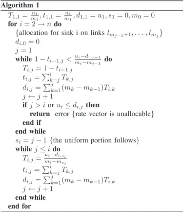
In [1] we define the following intra-session coding scheme which assigns the rate for each successive receiver as uni-formly as possible subject to capacity constraints imposed by assignments for previous receivers. This coding scheme resembles the water-filling process, as we allocate the packets of each receiver to the links in the upstream of the receiver equally as long as the links are not saturated by the previ-ous assignments. For a given rate vector (u1, u2, ..., un), we define a corresponding lower triangular n × n rate allocation matrix T , along with auxiliary variables ti,j ! "

i k=jTk,j, di,j! "

j

k=1(mk− mk−1)Ti,k, and si, by Algorithm 1: Note that Ti,si < Ti,si+1= Ti,si+2= ... = Ti,i.

Algorithm 1

T1,1= mu11, t1,1=

u1

m1, d1,1 = u1, s1= 0, m0= 0

for i = 2 → n do

{allocation for sink i on links lmj−1+1, . . . , lmj}

di,0= 0 j = 1

while 1 − ti−1,j <_mui_i−d_−mi,j−1

j−1 do Ti,j= 1 − ti−1,j ti,j=" i k=jTk,j di,j=" j k=1(mk− mk−1)Ti,k j ← j + 1 if j > i or ui≤ di,j then

return error {rate vector is unallocable} end if

end while

si= j − 1 {the uniform portion follows}

while j ≤ i do Ti,j= ui−di,si mi−msi ti,j="i_k=jTk,j di,j="j_k=1(mk− mk−1)Ti,k j ← j + 1 end while end for

Definition 3: A rate vector (u1, u2, ..., un) is called al-locable if Algorithm 1 does not return any error and the corresponding allocation matrix T is non-negative.

Definition 4: Given an allocable rate vector (u1, u2, ..., un), the “as uniform as possible” intra-session coding scheme is defined by the allocation

qji = Tj,k ∀i : mk−1< i ≤ mk. (4) Note that this coding scheme depends only on the rate vector !u and the set of deadlines.

We observe that under the “as uniform as possible” intrases-sion coding scheme the amount of information transmitted on the middle layer of the network is monotone:

Lemma 1: If (u1, u2, ..., un) is allocable, then the corre-sponding allocation matrix T satisfies:

Ti,j≤ Ti,j+1 ∀i, j : 1 ≤ i ≤ n, 1 ≤ j < i

Proof: See the appendix.

IV. MAINRESULT

We will verify the efficiency of the “as uniform as possible” intra-session coding scheme defined in Section III-B. The fol-lowing lemma states that under the sliding window erasure, the amount of the information loss is controlled by the parameter p for certain information allocations:

Lemma 2: Let A = {a1, a2, . . . , an} be an ordered set of nonnegative real numbers with a1 ≥ a2 ≥ . . . ≥ an and a1 = a2 = . . . = aT = a. Let ||X|| denote the sum of elements in an arbitrary finite set of real numbers X. Let B

be a (p, T )-unerased subset of A under some sliding window erasure with parameters p and T . Then,

||B||≥ (1 − p)||A||.

Proof: See the appendix.

Note that the monotonicity of the numbers ai is crucial as Lemma 1 states that the amount of the information allocated for a certain message Mi on the middle layer of the network is monotone under the “as uniform as possible” intrasession coding scheme. The following lemma establishes that the equally allocated part of a message has a length of at least T under the “as uniform as possible” intrasession coding for a constant multiple of a vector inside the capacity region of the network under the erasure-free case. Hence, by Lemma 2, the rate of the erased information for a particular message Mi will not be greater than p.

Lemma 3: Let V = {(v1, v2, . . . , vn)|" k

i=1vi ≤ mk ∀k : 1 ≤ k ≤ n}. Let !v ∈ V . The rate vector

1 1 + log(m1+T

m1 )

!v is achievable by the “as uniform as possible” intra-session coding, in a such way that the corresponding allocation q satisfies: qmi i−T +1= q i mi−T +2= . . . = q i mi ∀i : 1 ≤ i ≤ n. (5)

Proof: See the appendix.

Lemma 4 and Lemma 5 compares the capacity regions of the “as uniform as possible” intrasession coding scheme and any other coding scheme to an intermediate region V , which is the capacity region under the erasure-free case:

Lemma 4: Let U be the erasure correction capacity region

under some sliding window erasure with parameters p and T . Let V = {(v1, v2, . . . , vn)|"k_i=1vi ≤ mk ∀k : 1 ≤ k ≤ n}. Then

U ⊂ (1 − p + 1

T)V. (6)

Proof: See the appendix.

Lemma 5: Let W be the erasure correction capacity region

obtained by “as uniform as possible” intrasession coding under sliding window erasure with parameters p and T . Let V = {(v1, v2, . . . , vn)|" k i=1vi ≤ mk ∀k : 1 ≤ k ≤ n}. Then (1 − p) 1 1 + log(m1+T m1 ) V ⊂ W. (7)

Proof: See the appendix.

The following theorem states that the erasure correction capacity region of the “as uniform as possible” intra-session coding contains a constant multiple of that of any other coding scheme:

Theorem 1: Let U be the erasure correction capacity region

under sliding window erasure with parameters p and T . Let W be the erasure correction capacity region obtained by the “as uniform as possible” intrasession coding under sliding window erasure with parameters p and T . Then,

1 − p (1 + log(m1+T m1 ))(1 − p + 1 T) U ⊂ W. (8)

Proof: Applying Lemma 4 and Lemma 5, we obtain (8).

Let λ = sup{x ∈ R : xU ⊂ W }. As λ is the ratio of the two regions U and W , it measures how close the “as uniform as possible” intrasession coding scheme to the optimal coding scheme. Theorem 1 implies that

λ ≥ 1 − p (1 + log(m1+T m1 ))(1 − p + 1 T) . Note that for T ! 1, and m1! T we have

1 − p (1 + log(m1+T m1 ))(1 − p + 1 T) ≈ 1,

which implies that λ ≈ 1 for large values of T and large values of m1 compared to T .

APPENDIX

Proof of Lemma 1: Let’s prove the following statements

simultaneously by induction:

Ti,j≤ Ti,j+1 ∀i, j : 1 ≤ i ≤ n, 1 ≤ j < i, ti,j≥ ti,j+1 ∀i, j : 1 ≤ i ≤ n, 1 ≤ j < i.

# (9) The statements hold trivially for (i, j) = (1, 1). Let the statements hold for all (i, j) before (k, l) in lexicographical order. Let’s now verify in three cases that (9) is satisfied for (i, j) = (k, l):

Case(1): l < sk:

By construction, we have:

Tk,l= 1 − tk−1,l, Tk,l+1= 1 − tk−1,l+1, tk,l=tk,l+1= 1.

Clearly, tk,l ≤ tk,l+1. By induction hypothesis, we have tk−1,l≥ tk−1,l+1. Hence Tk,l= 1 − tk−1,l≤ 1 − tk−1,l+1= Tk,l+1. Case(2): l = sk: By construction, we have: Tk,l= 1 − tk−1,l< uk− dk,l−1 mk− ml−1 , (10) Tk,l+1 = uk− dk,l mk− ml ≤ 1 − tk−1,l+1. (11) Hence, tk,l= tk−1,l+ Tk,l= 1 ≥ tk−1,l+1+ Tk,l+1= tk,l+1. From (11) we get: Tk,l+1=uk− dk,l mk− ml =uk− dk,l−1− (ml− ml−1)Tk,l mk− ml . (12)

Using (10) we obtain:

Tk,l(mk− ml−1) < uk− dk,l−1. (13) Combining (12) and (13) we get:

Tk,l+1> Tk,l.

Case(3): l > sk:

By construction, we have:

Tk,l= Tk,l+1,

tk,l= Tk,l+ tk−1,l, tk,l+1= Tk,l+1+ tk−1,l+1. By induction hypothesis, tk−1,l≥ tk−1,l+1. Hence,

tk,l≥ tk,l+1.

Proof of Lemma 2: Let B = {ak1, ak2, . . . , akm}, where

k1< k2< . . . < km. Let q = 1−p. Let s be the largest integer satisfiying ks≤ T . Let’s prove by induction that

ak1+ ak2+ . . . + akr ≥ q(a1+ a2+ . . . + a$r_q%)

+(r − q.r

q/)a$rq%+1 (14)

is satisfied for any r with m ≥ r ≥ s. For r = s, we have s ! i=1 aki= sa = aq.s q/ + (s − q. s q/)a ≥ q(a1+ a2+ . . . + a$s q%) + (s − q. s q/)a$qs%+1.

Let (14) be satisfied for some r ≥ s. As kr+1> T , and B satisfies (1) we have r = |B ∩ {a1, a2, . . . , akr+1−1}|≥ (1 − p)(kr+1− 1) = q(kr+1− 1), which is equivalent to kr+1≤ 1 + r q. As kr+1 is an integer we have: kr+1≤ 1 + . r q/, which implies akr+1 ≥ a$r_q%+1. (15)

As ai is monotone, using (15) and the induction hypothesis we get r+1 ! i=1 aki≥q $r q% ! i=1 ai+ (r − q. r q/)a$rq%+1+ akr+1 =q $r q% ! i=1 ai+ (r + 1 − q. r q/)a$rq%+1 ≥q $r q%+1 ! i=1 ai+ (r + 1 − q. r + 1 q /)a$r+1 q %+1,

which means that (14) is satisfied for r + 1. Hence we established (14). As B satisfies (1), we have m = |B ∩ A| ≥ (1 − p)n = qn, which implies n ≤ .m q/. As (14) is satisfied for r = m, we have

||B|| = m ! i=1 aki≥ q(a1+ a2+ . . . + a$m_q%) ≥ q(a1+ a2+ . . . + an) = q||A|| = (1 − p)||A||, as desired.

Proof of Lemma 3: Let α = 1

1+log(m1+T_m1 ). As V is the capacity region under erasure-free case and α < 1, α!v is achievable by the “as uniform as possible” intra-session coding under the erasure-free case.

Assume to the contrary that (5) is not satisfied for some k ∈ {1, 2, . . . , n}. Without loss of generality, we may assume that k is the smallest such integer. Then we have

k ! i=1 qi j= 1, ∀j : 1 ≤ j ≤ mk− T. (16) Using (16), we get: αmk≥ k ! i=1 αvi= mk ! j=1 k ! i=1 qi j≥ mk−T ! j=1 k ! i=1 qi j = mk− T, which implies: mk≤ T 1 − α. (17)

Let’s first prove that

mk < m1+ 2T. (18) Using (17), we get mk ≤ T 1 − α = T 1 − 1 1+log(m1+T_m1 ) = T (1 + log( m1+T m1 )) log(m1+T m1 ) .

Hence it is enough to show that T (1 + log(m1+T m1 )) log(m1+T m1 ) < m1+ 2T. (19) Let x = T

m1. Then, (19) is equivalent to:

g(x) = (1 + 1

x) log(1 + x) > 1, (20) which follows immediately by the fact that g&_{(x) > 0 and} limx→0g(x) = 1.

Let t be the smallest integer satisfying mt ≥ mk− T + 1. Hence,

mt−1≤ mk− T. (21)

Let s be the smallest integer satisfying s+1 ! i=1 αvi mi ≥ 1. (22) Let X = v1+ v2+ . . . + vt−1, Y = v1+ v2+ . . . + vs+1. Using (22) we get: 1 ≤ s+1 ! i=1 αvi mi < α + $Y %−m1 ! i=1 α m1+ i +α(Y − .Y /) Y < α  1 + $Y %−m1 ! i=1 1 m1+ i +(Y − .Y /) Y   < α ( 1 + log(Y m1 ) ) . Hence, Y > m1+ T. (23) As ms+1≥ Y , (18), (21) and (23) implies: ms+1≥ Y > m1+ T ≥ mk− T + 1 > mt−1, which implies: s + 1 ≥ t.

Let pidenote the length of the uniform block for i-th receiver. Let r = mk− T + 1. By assumption, pk< T , which implies:

k−1 ! i=t qri+ αvk T > 1. (24) As pi ≥ T for i ∈ {1, 2, . . . , k − 1}, and qri ≤ αvi/pi, (24) implies: 1 < k−1 ! i=t qri+ αvk T = s ! i=t αvi mi + k−1 ! i=s+1 qir+ αvk T ≤ s ! i=t αvi mi + qrs+1+ k−1 ! i=s+2 αvi pi +αvk T ≤ s ! i=t αvi mi + qrs+1+ k ! i=s+2 αvi T . Let S ="s i=t αvi mi + q s+1 r + "k i=s+2 αvi T . Let’s maximize S under the condition (22). As increasing vs+2 and decreasing vs+1 at the same amount increases S, we may assume that equality is satisfied in (22), i.e.

s+1 ! i=1 vi mi = 1 α= 1 + log( m1+ T m1 ). (25) Hence S = s+1 ! i=t αvi mi + k ! i=s+2 αvi T ≥ 1. (26) Let h(v1, v2, . . . , vn) = s+1 ! i=t vi mi + k ! i=s+2 vi T. Let’s prove that

h(v1, v2, . . . , vn) ≤ 1

α= 1 + log( m1+ T

m1 ), (27)

which will contradict (26). As h(v1, v2, . . . , vn) ≤ s+1 ! i=t vi mi +mk− Y T ,

in order to verify (27), it is enough to show that s+1 ! i=t vi mi +mk− Y T ≤ 1 α. (28)

Using (25), (28) is equivalent to: T t−1 ! i=1 vi mi + Y ≥ mk. (29) Let β = t−1 ! i=1 vi mi . Then, clearly X = t−1 ! i=1 vi≥ m1 t−1 ! i=1 vi mi = m1β, (30) Y − X = s+1 ! i=t vi≥ mt s+1 ! i=t vi mi = mt( 1 α− β). (31)

We will consider two cases:

Case (1): mt≥ m1+ T . Using (30) and (31), we get:

T t−1 ! i=1 vi mi + Y = T β + X + Y − X ≥ T β + m1β + (1 α− β)mt ≥ T β + m1β + ( 1 α− β)(m1+ T ) =m1+ T α ≥ m1+ 2T, (32)

where the last inequality is equivalent to log(1+t) ≥ t t+1 after setting t = T /m1, hence follows from the inequality (20). As (32) implies (29), and (29) is equivalent to (27), we get a contradiction. Case (2): mt< m1+ T . If β ≥ 1, as Y ≥ m1+ T , we have T t−1 ! i=1 vi mi + Y = T β + Y ≥ m1+ 2T ≥ mk, which establishes (29). Hence we get a contradiction. We may assume that β < 1. Using (23), we have Y > m1+ T > mt. Hence 1 α− β = s+1 ! i=t vi mi ≤mt− X mt + log(Y mt ), which is equivalent to:

Y ≥ mte

1 α−β+

X

mt−1_{. (33)}

Using (30) and (33), we get: T t−1 ! i=1 vi mi + Y = T β + Y ≥ T β + mte 1 α−β+ X mt−1 ≥ T β + mte 1 α−β+m1βmt −1 = T β + mte1+log(1+ T m1)−β+m1βmt −1 = T β + mt(1 + T m1 )eβ(m1mt−1). (34) Let f (x) = T x + mt(1 +_mT 1)e x(m1_mt−1)_{. Then,} f&(x) = T + mt(1 + T m1)( m1 mt − 1)ex(m1mt−1) ≥ T + mt(1 + T m1 )(m1 mt − 1) = T + (1 + T m1 )(m1− mt). (35) If T + (1 + T m1)(m1− mt) ≤ 0, using (34) and (35) we get: T t−1 ! i=1 vi mi + Y ≥ f (β) ≥ f (0) + β[T + (1 + T m1 )(m1− mt)] = mt(1 + T m1 ) + β[T + (1 + T m1 )(m1− mt)] ≥ mt(1 + T m1) + [T + (1 + T m1)(m1− mt)] = m1+ 2T ≥ mk,

which establishes (29). Hence we get a contradiction. If T + (1 + T

m1)(m1− mt) > 0, using (34) and (35) we get:

T t−1 ! i=1 vi mi + Y ≥ f (β) ≥ f (0) = mt(1 + T m1 ) ≥ mt+ T ≥ mk, which establishes (29), again we get a contradiction.

Proof of Lemma 4: As U ⊂ V , if p ≤ _T1, then clearly U ⊂ (1 − p +_T1)V .

Let p > _T1. Define q = 1 − p +_T1. Define Z ⊂ I as

|Z ∩ {l1, l2, . . . , lk}| = .qk/ ∀k : 1 ≤ k ≤ mk. As 0 ≤ q < 1, Z is well-defined and unique. Let’s prove that Z is a (p, T )-unerased subset of I. Let t ≥ T and 0 ≤ i ≤ mn− t. We have:

|Z ∩ {li+1, ai+2, . . . , li+t}| = .q(i + t)/ − .qi/ > q(i + t) − qi − 1 = (1 − p + 1

T)t − 1 ≥ (1 − p)t,

as desired.

Let (u1, u2, . . . un) ∈ U . Applying cut-set bounds for Z, we have:

k ! i=1

ui≤ |Z ∩ {l1, l2, . . . , lmk}| = .qmk/ ≤ qmk,

which implies that U ⊂ qV = (1 − p + 1

T)V , as desired.

Proof of Lemma 5: Let !v ∈ V . Let α = 1 1+log(m1+T

m1 )

. By Lemma 3, the rate vector α!v is achievable by the “as uniform as possible” intra-session coding in a such way that the corresponding allocation q satisfies:

qimi−T +1= q i mi−T +2= . . . = q i mi ∀i : 1 ≤ i ≤ n. Let Qi = {qmi i, q i mi−1, . . . , q i 1}. We know that qimi ≥ qi mi−1 ≥ . . . ≥ q i

1. Let Q&i be a (p, T )-unerased subset of Qi. By Lemma 2:

||Q&

i||≥ (1 − p)||Qi|| = (1 − p)αvi. Hence (1 − p)α!v∈ W , which establishes (7).

REFERENCES

[1] O. Tekin, S. Vyetrenko, T. Ho, and H. Yao, “Erasure correction for nested receivers,” in Allerton conference on Communication, Control, and

Computing, September 2011.

[2] E. Martinian and C.-E.Sundberg, “Burst erasure correction codes with low decoding delay,” IEEE Trans. Inf. Theory, vol. 50, no. 10, pp. 2494–2502, October 2005.

[3] E. Martinian and M. Trott, “Delay-optimal burst erasure code construc-tion,” in ISIT, July 2007.