Object detection using optical and lidar data fusion with graph-cuts

(1)

OBJECT DETECTION USING OPTICAL

AND LIDAR DATA FUSION WITH

GRAPH-CUTS

a thesis submitted to

the graduate school of engineering and science

of bilkent university

in partial fulfillment of the requirements for

the degree of

master of science

in

computer engineering

By

Onur Ta¸sar

March 2017

(2)

OBJECT DETECTION USING OPTICAL AND LIDAR DATA FUSION WITH GRAPH-CUTS

By Onur Ta¸sar March 2017

We certify that we have read this thesis and that in our opinion it is fully adequate, in scope and in quality, as a thesis for the degree of Master of Science.

Selim Aksoy(Advisor)

Aydın Alatan

Ramazan G¨okberk Cinbi¸s

Approved for the Graduate School of Engineering and Science:

Ezhan Kara¸san

(3)

ABSTRACT

OBJECT DETECTION USING OPTICAL AND LIDAR

DATA FUSION WITH GRAPH-CUTS

Onur Ta¸sar

M.S. in Computer Engineering Advisor: Selim Aksoy

March 2017

Object detection in remotely sensed data has been a popular problem and is commonly used in a wide range of applications in domains such as agricul-ture, navigation, environmental management, urban monitoring and mapping. However, using only one type of data source may not be sufficient to solve this problem. Fusion of aerial optical and LiDAR data has been a promising ap-proach in remote sensing as they carry complementary information for object detection. We propose frameworks that partition the data in multiple levels and detect objects with minimal supervision in the partitioned data. Our method-ology involves thresholding the data according to height, and dividing the data into smaller components to process it efficiently in the preprocessing step. For the classification task, we propose two graph cut based procedures that detect objects in each component using height information from LiDAR, spectral in-formation from aerial data, and spatial inin-formation from adjacency maps. The first procedure provides a binary classification, whereas the second one performs a multi-class classification. We use the first framework to separate buildings from trees in the high pixels, and roads from grass areas in the low pixels. The second procedure is used to detect all of the classes in each component at once.

The only supervision our proposed methodology requires consists of samples that are used to estimate the weights of the edges in the graph for the graph-cut procedures. Experiments using a benchmark data set show that the performance of the proposed methodology that uses small amount of supervision is compatible with the ones in the literature.

(4)

¨

OZET

C

¸ ˙IZG ˙E KES˙IT ˙ILE OPT˙IK VE LIDAR VER˙I VER˙I

F ¨

UZYONU KULLANARAK NESNE TESP˙IT˙I

Onur Ta¸sar

Bilgisayar M¨uhendisli˘gi, Y¨uksek Lisans Tez Danı¸smanı: Selim Aksoy

Mart 2017

Uzaktan algılama verisinde nesne tespiti, olduk¸ca popüler bir problem olmu¸stur ve tarım, navigasyon, ¸cevre düzenlemesi, kentsel görüntüleme ve haritacılık gibi ¸cok geni¸s bir yelpazedeki uygulama alanlarında yaygın olarak kullanılmaktadır. Fakat bu problemi ¸cözmek i¸cin sadece tek bir veri kayna˘gını kullanmak yeterli olmaya-bilir. Havadan ¸cekilmi¸s optik ve LiDAR verilerinin füzyonu, birbirini tamam-layıcı bilgiler ta¸sıdı˘gı i¸cin uzaktan algılama verisinde nesne tespitinde umut verici bir yakla¸sım olmu¸stur. Biz verinin ¸coklu düzey bölünmesini ger¸cekle¸stiren ve bölünmü¸s veriyi minimum düzeyde ö˘grenme kullanarak nesneleri tespit eden sis-temler öneriyoruz. Yöntemimiz ön i¸sleme a¸samasında veriyi yükseklik de˘gerine göre e¸sikleme ve daha etkili bir bi¸cimde i¸slemek i¸cin onu kü¸cük bile¸senlere bölme adımları i¸ceriyor. Sınıflandırma görevi i¸cin ise, LiDAR verisinden yükseklik, havadan ¸cekilmi¸s veriden spektral ve kom¸suluk haritasından konumsal bilgileri kullanarak, her bir bile¸sende nesneleri tespit eden iki farklı ¸cizge kesme tabanlı yöntem öneriyoruz. ˙Ilk yöntem ikili sınıflandırma sa˘glarken, ikincisi ise ¸coklu sınıflandırma ger¸cekle¸stiriyor. ˙Ilk yöntemi kullanarak yüksek piksellerde binaları a˘ga¸clardan, al¸cak piksellerde ise yolları ¸cimenlik alanlardan ayırt ediyoruz. ˙Ikinci yöntem ise her bir bile¸sendeki bütün nesneleri tek seferde tespit etmek i¸cin kul-lanılıyor.

Bizim önerdi˘gimiz yöntemin ihtiya¸c duydu˘gu tek ö˘grenme ¸cizge kesme yöntemindeki ¸cizgenin kenarlarının a˘gırlıklarını belirlemek i¸cin kullanılan ¨

orneklerdir. Bir kıyas veri seti ¨uzerinde ger¸cekle¸stirilen deneyler g¨osteriyor ki ¨

onerdi˘gimiz az miktarda ö˘grenme kullanan yöntem literatürdeki sonu¸clarla uyum-ludur.

(5)

Acknowledgement

First of all, I would like to express my gratitude to my supervisor Assoc. Prof. Selim Aksoy for his motivation and encouragement throughout my master’s ed-ucation. Without his guidance and assistance, this thesis would not have been possible.

I also appreciate Asst. Prof. Ramazan G¨okberk Cinbi¸s and Prof. Aydın Alatan for their feedback and constructive comments on my thesis.

I thank to my friends at Bilkent; Ali Burak Ünal, Barı¸s Ge¸cer, Bülent Sarıyıldız, Can Fahrettin Koyuncu, Caner Mercan, Gencer Sümbül, Iman Dezn-aby, Noushin Salek Faramarzi, Troya Ç a˘gıl Köylü and others for all the enjoyable moments.

I also would like to thank to my best friends Can Altu˘ger and Semo for their amazing companionship and valuable emotional support when I need most. I will never forget the enjoyable and unforgettable time we have had together.

Most importantly, I am so lucky to have a wonderful, caring and supportive family. I am grateful to my beloved father Süleyman Ta¸sar, mother Fadime Ta¸sar, sister Özlem Ta¸sar and brother Özgür Ta¸sar for their endless support and love. None of my achievements would have been possible without them.

Finally, as a Turkish prospective scientist, my sincere gratitude goes to Mustafa Kemal Atatürk, who showed us that science is the most reliable guide for civiliza-tion, for life, for success in the world. I dedicate this scientific contribution to my father Süleyman Ta¸sar, my mother Fadime Ta¸sar and the great leader Mustafa Kemal Atatürk!

This work was supported in part by the BAGEP Program of the Science Academy.

(6)

1.1 Motivation and Problem Definition . . . 1 1.2 Contribution . . . 3 1.3 Outline . . . 4 2 Related Works 5 3 Methodology 12 3.1 Data set . . . 12 3.2 Overview . . . 14 3.3 Preprocessing . . . 15 3.3.1 Grayscale Reconstruction Based on Geodesic Dilation . . . 16 3.3.2 Progressive Morphological Filtering . . . 17 3.3.3 Area Opening . . . 19 3.3.4 Opening . . . 20

(7)

CONTENTS vii

3.3.5 Generation of the Connected Components . . . 21

3.4 Features . . . 22

3.4.1 Spectral Features . . . 22

3.4.2 Height Features . . . 24

3.5 Graph Cuts . . . 25

3.5.1 Max-flow/Min-cut Procedure . . . 25

3.5.2 Multi-label Optimization Procedure . . . 32

4 Experiments 38 4.1 Experimental Setup . . . 38 4.2 Evaluation Criteria . . . 39 4.3 Parameter Selection . . . 41 4.4 Results . . . 43 4.5 Discussion . . . 69 5 Conclusion 78

(8)

List of Figures

3.1 An example area from the data set. (a) Ortho photo. (b) DSM. (c) Reference data with class labels: impervious surfaces (white), building (blue), low vegetation (cyan), high vegetation (green), car (yellow). . . 13 3.2 Flowchart of the proposed method that is based max-flow/min-cut. 15 3.3 Flowchart of the proposed method that is based on multi-label

optimization. . . 16 3.4 Flowchart of the Gray-scale Reconstruction. Top-left image: I is

the mask image (DSM), I-h corresponds to J, which is the marker image, Top-right image: reconstructed image (DTM), bottom im-age: difference between the DSM and DTM (NDSM). This figure was taken from [1]. . . 18 3.5 Illustration for the progressive morphological filtering algorithm.

I1 and I2 are sizes of the structuring elements, dhmax(t),1 and

dhmax(t),2 are the height thresholds in the first and second

iter-ations, and dhp,1 is difference between the height of the pixel P in

the original DSM image and the height of the same pixel in the opened image at the end of the first iteration. This figure was taken from [2]. . . 19

(9)

LIST OF FIGURES ix

3.6 Illustration of NDSM generation using area opening. (a) DSM, (b) DTM obtained by using area opening, (c) NDSM generated by subtracting DTM from DSM. Each image in the figure has been normalized between 0-255 for better visualization. . . 20 3.7 Illustration of DSM generation using opening. (a) DSM, (b) DTM

obtained by using opening, (c) NDSM generated by subtracting DTM from DSM. For the sake of visualization purposes, each image in this figure is normalized between 0 and 255. . . 21 3.8 Example binary masks, and their connected components. (a) Mask

for the high pixels, (b) Mask for the low pixels, (c) Connected components of the high mask, (d) Connected components of the low mask. . . 23 3.9 An example infrared ortho photo image and its corresponding

fea-ture intensity maps. (a) Infrared image, (b) NDVI map, (c) Irreg-ularity map. . . 25 3.10 An example graph model for the max-flow/min-cut procedure. . . 26 3.11 Histograms and the estimated probability distributions of each

class for the NDVI feature. NDVI values are modeled using Gaus-sian mixture models with 4 components. (a) road, (b) building, (c) grass and (d) tree. . . 29 3.12 Histograms and the estimated probability distributions of each

class for the irregularity feature. The irregularity values are mod-eled using Exponential models. (a) road, (b) building, (c) grass and (d) tree. . . 30

(10)

LIST OF FIGURES x

3.13 Histograms and the estimated probability distributions of each class for the height feature. Height values of roads, grass and trees are modeled using Exponential models, and height values of build-ings are modeled by a Gaussian mixture model with 4 components. (a) road, (b) building, (c) grass and (d) tree. . . 31 3.14 Histogram and the estimated probability distribution for the

dis-tances between two neighboring pixels. The disdis-tances are modeled using Exponential fit. . . 32 3.15 Posterior probability map of each class for the ndvi feature. (a)

road, (b) building, (c) grass and (d) tree. . . 33 3.16 Posterior probability map of each class for the irregularity feature.

(a) road, (b) building, (c) grass and (d) tree. . . 34 3.17 Posterior probability map of each class for the height feature. (a)

road, (b) building, (c) grass and (d) tree. . . 35 3.18 Posterior probability distributions of each class for (a) NDVI, (b)

irregularity, (c) height. . . 36

4.1 Aerial data of the whole Vaihingen region and the selected areas. . 45 4.2 DSM data of the whole Vaihingen region and the selected areas. . 46 4.3 Group 1, area 5. (a) Aerial, (b) Ground-truth, (c) DSM, (d) DTM,

(e) NDSM, (f) Connected components. . . 47 4.4 Group 1, area 15. (a) Aerial, (b) Ground-truth, (c) DSM, (d)

DTM, (e) NDSM, (f) Connected components. . . 48 4.5 Group 1, area 37. (a) Aerial, (b) Ground-truth, (c) DSM, (d)

(11)

LIST OF FIGURES xi

4.6 Group 2, area 3. (a) Aerial, (b) Ground-truth, (c) DSM, (d) DTM, (e) NDSM, (f) Connected components. . . 50 4.7 Group 2, area 11. (a) Aerial, (b) Ground-truth, (c) DSM, (d)

DTM, (e) NDSM, (f) Connected components. . . 53 4.10 Group 3, area 1. (a) Aerial, (b) Ground-truth, (c) DSM, (d) DTM,

(e) NDSM, (f) Connected components. . . 54 4.11 Group 3, area 7. (a) Aerial, (b) Ground-truth, (c) DSM, (d) DTM,

(e) NDSM, (f) Connected components. . . 55 4.12 Group 3, area 28. (a) Aerial, (b) Ground-truth, (c) DSM, (d)

DTM, (e) NDSM, (f) Connected components. . . 56 4.13 Results for group 1, area 5. (a) Ground-truth, (b)

Max-flow/min-cut, constant smoothness cost, (c) Max-flow/min-Max-flow/min-cut, adaptive smoothness cost, (d) Multi-label optimization, constant smooth-ness cost, (e) Multi-label optimization, adaptive smoothsmooth-ness cost. 57 4.14 Results for group 1, area 15. (a) Ground-truth, (b)

Max-flow/min-cut, constant smoothness cost, (c) Max-flow/min-Max-flow/min-cut, adaptive smoothness cost, (d) Multi-label optimization, constant smooth-ness cost, (e) Multi-label optimization, adaptive smoothsmooth-ness cost. 59

(12)

LIST OF FIGURES xii

4.16 Results for group 2, area 3. (a) Ground-truth, (b) Max-flow/min-cut, constant smoothness cost, (c) Max-flow/min-Max-flow/min-cut, adaptive smoothness cost, (d) Multi-label optimization, constant smooth-ness cost, (e) Multi-label optimization, adaptive smoothsmooth-ness cost. 60 4.17 Results for group 2, area 11. (a) Ground-truth, (b)

Max-flow/min-cut, constant smoothness cost, (c) Max-flow/min-Max-flow/min-cut, adaptive smoothness cost, (d) Multi-label optimization, constant smooth-ness cost, (e) Multi-label optimization, adaptive smoothsmooth-ness cost. 66

(13)

LIST OF FIGURES xiii

4.23 Zoomed example 1. (a) Aerial data, (b) DSM, (c) Ground-truth, (d) flow/min-cut with constant smoothness output, (e) Max-flow/min-cut with adaptive smoothness output, (f) Multi-label op-timization with constant smoothness output, (g) Multi-label opti-mization with adaptive smoothness output. . . 72 4.24 Zoomed example 2. (a) Aerial data, (b) DSM, (c) Ground-truth,

(d) flow/min-cut with constant smoothness output, (e) Max-flow/min-cut with adaptive smoothness output, (f) Multi-label op-timization with constant smoothness output, (g) Multi-label opti-mization with adaptive smoothness output. . . 73 4.25 Zoomed example 3. (a) Aerial data, (b) DSM, (c) Ground-truth,

(d) flow/min-cut with constant smoothness output, (e) Max-flow/min-cut with adaptive smoothness output, (f) Multi-label op-timization with constant smoothness output, (g) Multi-label opti-mization with adaptive smoothness output. . . 75

(14)

LIST OF FIGURES xiv

4.28 Zoomed example 6. (a) Aerial data, (b) DSM, (c) Ground-truth, (d) flow/min-cut with constant smoothness output, (e) Max-flow/min-cut with adaptive smoothness output, (f) Multi-label op-timization with constant smoothness output, (g) Multi-label opti-mization with adaptive smoothness output. . . 76 4.29 Zoomed example 7. (a) Aerial data, (b) DSM, (c) Ground-truth,

(d) flow/min-cut with constant smoothness output, (e) Max-flow/min-cut with adaptive smoothness output, (f) Multi-label op-timization with constant smoothness output, (g) Multi-label opti-mization with adaptive smoothness output. . . 77

(15)

List of Tables

4.1 Data division for the 3-Fold cross validation. . . 40 4.2 Parameters for dividing the data into two groups as high and low. 42 4.3 The best values for λs in the cost function of the max-flow/min-cut

for the high pixels. . . 42 4.4 The best values for λs in the cost function of the max-flow/min-cut

for the low pixels. . . 42 4.5 The best values for λs in the cost function of the multi-label

opti-mization. The parameters are divided by 1000. . . 43 4.6 Pixel-based overall F1-scores calculated from Tables A.7, A.8, A.9

and A.10. Method 1 and method 2 are max-flow/min-cut with con-stant and adaptive smoothness costs, and method 3 and method 4 are multi-label optimization with constant and adaptive smooth-ness costs. . . 67 4.7 Object-based overall F1-scores calculated from A.11, A.12, A.13

and A.14. Method 1 and method 2 are max-flow/min-cut with con-stant and adaptive smoothness costs, and method 3 and method 4 are multi-label optimization with constant and adaptive smooth-ness costs. . . 67

(16)

LIST OF TABLES xvi

4.8 Pixel-based overall recall values calculated from pixel-based confu-sion matrices in Tables A.1, A.2 and A.3. Method 1 and method 2 are max-flow/min-cut with constant and varying smoothness costs, and method 3 and method 4 are multi-label optimization with con-stant and varying smoothness costs. . . 67 4.9 Object-based overall recall values calculated from object-based

confusion matrices in Tables A.4, A.5 and A.6. Method 1 and method 2 are max-flow/min-cut with constant and varying smooth-ness costs, and method 3 and method 4 are multi-label optimiza-tion with constant and varying smoothness costs. . . 68 4.10 Overall accuracies calculated from pixel-based confusion matrices

in Tables A.1, A.2 and A.3. . . 68 4.11 Overall accuracies calculated from object-based confusion matrices

in Tables A.4, A.5 and A.6. . . 68 4.12 Abbreviations of the methods whose results are submitted to the

ISPRS, and their corresponding references. . . 70 4.13 ISPRS F1-score results table. . . 71

A.1 Pixel-based confusion matrices for group 1. (a) Max-flow/min-cut with constant smoothness cost, (b) Max-flow/min-Max-flow/min-cut with adaptive smoothness cost, (c) Multi-label optimization with con-stant smoothness cost, (d) Multi-label optimization with adaptive smoothness cost. . . 91 A.2 Pixel-based confusion matrices for group 2. (a)

Max-flow/min-cut with constant smoothness cost, (b) Max-flow/min-Max-flow/min-cut with adaptive smoothness cost, (c) Multi-label optimization with con-stant smoothness cost, (d) Multi-label optimization with adaptive smoothness cost. . . 92

(17)

LIST OF TABLES xvii

A.3 Pixel-based confusion matrices for group 3. (a) Max-flow/min-cut with constant smoothness cost, (b) Max-flow/min-Max-flow/min-cut with adaptive smoothness cost, (c) Multi-label optimization with con-stant smoothness cost, (d) Multi-label optimization with adaptive smoothness cost. . . 93 A.4 Object-based confusion matrices for group 1. (a)

Max-flow/min-cut with constant smoothness cost, (b) Max-flow/min-Max-flow/min-cut with adaptive smoothness cost, (c) Multi-label optimization with con-stant smoothness cost, (d) Multi-label optimization with adaptive smoothness cost. . . 94 A.5 Object-based confusion matrices for group 2. (a)

Max-flow/min-cut with constant smoothness cost, (b) Max-flow/min-Max-flow/min-cut with adaptive smoothness cost, (c) Multi-label optimization with con-stant smoothness cost, (d) Multi-label optimization with adaptive smoothness cost. . . 95 A.6 Object-based confusion matrices for group 3. (a)

Max-flow/min-cut with constant smoothness cost, (b) Max-flow/min-Max-flow/min-cut with adaptive smoothness cost, (c) Multi-label optimization with con-stant smoothness cost, (d) Multi-label optimization with adaptive smoothness cost. . . 96 A.7 Pixel-based F1 scores for the results obtained by max-flow/min-cut

with constant smoothness cost. . . 97 A.8 Pixel-based F1 scores for the results obtained by max-flow/min-cut

with adaptive smoothness cost. . . 98 A.9 Pixel-based F1 scores for the results obtained by multi-label

opti-mization with constant smoothness cost. . . 99 A.10 Pixel-based F1 scores for the results obtained by multi-label

(18)

LIST OF TABLES xviii

A.11 Object-based F1 scores for the results obtained by max-flow/min-cut with constant smoothness cost. . . 101 A.12 Object-based F1 scores for the results obtained by

max-flow/min-cut with adaptive smoothness cost. . . 102 A.13 Object-based F1 scores for the results obtained by multi-label

op-timization with constant smoothness cost. . . 103 A.14 Object-based F1 scores for the results obtained by multi-label

(19)

Chapter 1 Introduction

1.1 Motivation and Problem Definition

With the continuous advancements in satellite sensors, it is now possible to cap-ture massive amount of remote sensing data having very high spatial resolution, as well as rich spectral information. Having such a huge, very high resolution data has opened the door to various remote sensing applications but at the same time it has made the processing operation harder. Object detection has been one of the most popular problems in remote sensing applications, and has been studied extensively for several decades because a good solution for this problem is crucial for a wide range of very important applications in domains such as agriculture, navigation, environmental management, urban monitoring and mapping. A good methodology for this problem has to detect the objects effectively and efficiently. In traditional classification methods, each pixel is classified by using only spectral information, where the spatial information is ignored. However, in [3, 4, 5, 6, 7] it is proved that using object-based classification methods, where spatially similar pixels are grouped into an object, achieve more satisfactory re-sults than using traditional pixel-based classification algorithms. The main rea-son why pixel-wise techniques perform worse is that since each pixel is processed

(20)

independently, the resulting label map becomes spatially incoherent in most of the cases. On the contrary, using spatial information alone is also not suitable for classification problems because semantic information of the pixels is lost if the spectral information is totally ignored. For these reasons, both spectral and spatial information definitely need to be used.

There are a lot of published papers that are related to spatial-spectral image classification. To give a few examples, in [8] extended multi-attribute profiles, which represent effectively the spatial and spectral information of hyper-spectral images are used as the features. A kernel is created using multiple kernel learning approach and given to an SVM classifier to generate a semantic labeling from the given image. In [9] in order to respect spatial coherency, the neighboring pixels of each pixel in a w × w window is found and a box of size w × w × n, where n is number of channels, is created for each pixel. 1-D vectors that have been obtained by flattening the boxes and the spectrum vectors of the hyper-spectral image are fed into a Deep Belief Network (DBN) structure to classify the image. In [10] instead of converting spatial features to 1-D vectors as in most of the papers, they propose a matrix representation for the features to preserve the spatial coherency. Pixels are classified with the SVM that takes the important features that are selected from the matrix representation with their proposed matrix-based discriminant analysis method. Spatial-spectral hybrid features are extracted by applying spectral-spatial cross-correlation constraint method to both spectral values and spatial adjacency, and the data are classified using a random forest classifier in [11].

Due to the increasing level of detail in the spectral bands of the optical im-ages, using only color information as features for object detection may not be sufficiently discriminative because colors of pixels belonging to the same object may have very high variations. In addition, shadows falling onto objects make the detection task even more challenging. Since the works described above use only color information, they may fail to detect the objects that are in shadowed areas. In addition to the high resolution optical satellite and aerial imagery, more recently, developments in the Light Detection and Ranging (LiDAR) technology and LiDAR’s capability of storing 3D shapes in the real world as point clouds

(21)

have enabled grid based digital surface models (DSM) that are generated from the point clouds as additional data sources. Consequently, exploiting both color and height information together by fusing aerial optical and DSM data has been a popular problem in remote sensing image analysis.

1.2 Contribution

In this thesis, we study the object detection problem for remote sensing data by using spatial, spectral and height information. We propose hierarchical frame-works to solve this problem. We use both aerial data, which provide spectral information, and LiDAR based DSMs, where height information of each pixel is stored. We first remove all objects from the DSMs by using morphological op-erations to estimate the bare ground. The resulting data are called the digital terrain model (DTM). Then, we subtract the DTMs from the DSMs to generate another data, which store relative height information of each pixel above the es-timated ground, and called the normalized digital surface model (NDSM). Our hierarchical framework starts by partitioning the data set into two as high and low by thresholding the NDSMs. We then find the connected components in both high and low binary masks that represents this partitioning. This reduces the computational complexity because the connected components that are processed separately are much more smaller than the whole very high resolution input data. The main computational tool in this thesis is a graph-cut framework that fuses the spectral information from aerial data, height information from DSMs, and spa-tial information from neighborhood maps. Minimal supervision, where training data are used for estimating class-conditional probabilities to determine weight of the edges in the neighborhood maps, is used. Graph-cut procedure performs a pixel-wise classification but it forces the neighboring pixels to have the same label so that the resulting classification map becomes spatially coherent. We propose to use two frameworks, where the first framework is based on a max-flow/min cut algorithm [12, 13] and the second one is based on multi-label optimization [14, 15, 16]. In the first framework, we apply the max-flow/min-cut algorithm to high pixels to detect buildings and trees, and to low pixels to find roads and grass

(22)

areas. Then, we merge the classification maps coming from the low and the high pixels to get only one classification map. In the second framework, we apply the multi-label optimization algorithm to each connected component to detect all of the classes in the given data. The main contribution of this thesis is the use of these graph cut frameworks for fusion of spectral, height and spatial information for object detection with minimal supervision. Finally, extensive quantitative and qualitative experiments, where different types of areas are used in a benchmark data set, are done to evaluate performance of our frameworks. Although we use only small amount of supervision, our results are compatible with the ones in the literature.

Some part of this work was published as [17].

1.3 Outline

In Chapter 2, we introduce the related works that use spatial, spectral and height information in order to classify the remote sensing data.

In Chapter 3, we first describe the data set used in this thesis in great detail. We then provide an overview about the two proposed frameworks. Then, we explain how we generate the relative height information of each pixel from the raw elevation data and how we divide the data into smaller components to process it efficiently. Finally, we explain the features we extract from both aerial and LiDAR data, and the graph cut procedures in detail.

In Chapter 4, firstly, we describe the experimental setup, then, explain eval-uation criteria and how we optimize the parameters. We provide both numeric and visual results, and give a detailed discussion at the end of this chapter.

(23)

Chapter 2 Related Works

Since the most common object class in remote sensing applications is building, there are lots of papers trying to solve the building detection problem using spa-tial, spectral and height information. Almost all of the approaches start with dividing the data into two groups as high and low by thresholding the LiDAR data. Then, the low pixels are ignored and buildings are detected in the high pixels. In [18], a threshold is applied to the high pixels to eliminate the trees covering low area. Then, buildings are separated from the remaining trees by taking advantage of edge histograms. However, all of the buildings are assumed to a have rectangular shape, which may not be always the case. A probabilistic framework that is based on conditional random fields (CRF) is proposed in [19]. In [20, 21], after dividing the data into two in the preprocessing step, buildings are separated from the remaining trees by using traditional machine learning meth-ods. The method described in [21] can also detect trees. A stratified morphology based approach is described in [22]. Firstly, potential buildings are extracted using the proposed morphological building index (MBI) method and they are post-processed by morphological operations. However, obviously, the biggest dis-advantage of these algorithms is that they have been designed to detect only one class. In real life problems, there are more than one class in remote sensing data. Among the methods that are able to detect more than one class, rule based

(24)

approaches are very popular. Most of the published works using rule based ap-proaches use height and NDVI as the features because NDVI is a distinctive feature for the healthy vegetation, and height is a good feature to separate the high objects such as buildings and trees from the low ones such as grass areas and roads. Objects are detected by setting several thresholds for these features. The input data are segmented by applying a region growing method to the LiDAR data in [23]. Small regions are assumed to belong to tree class because the pixels belonging to trees tend to show high height variance. The remaining classes are detected by setting thresholds for certain features such as NDVI. In [24, 25, 26], lots of thresholds are set for height and NDVI features to detect objects. In [26], additional features such as the Enhanced Shadow Index (ESI) are also used. In [24], different thresholds are also determined to detect the objects belonging to the same class but located in shadowed and open areas. Finally borders of buildings are straightened by Hough transform. An object based classification approach, which generates a segmentation first and classifies each region of the segmentation map later, is proposed in [27, 28]. The segmentation map is gen-erated by watershed in the former paper, and it is gengen-erated by the quad-tree algorithm in combination of region growing in the latter paper. In [27], the in-put image is classified two different ways that are based on Gaussian Mixture Models and class specific rules. In [28], apart from the NDVI and height, a lot of additional features such as brightness and slope are also used. In [29], roads and buildings are detected with the rules defined in the paper, and the rest of the classes are found by an SVM classifier. A hierarchical rule tree is defined in [30] to detect the objects. Classification of the hyper-spectral and LiDAR data is performed separately in [31], and these two classification maps are combined with the defined rule chains. However, the rule chains of these methods might be data specific and may fail to detect objects when new data comes.

Deep neural network based approaches are also very popular in detecting ob-jects by using spatial, spectral and height information. In [32], various extinction profiles are extracted from both the hyper-spectral and LiDAR data and used as the features. Then, these features are combined together with several feature

(25)

fusion methods such as vector stacking and graph based methods. The fused fea-tures are given to a deep convolutional structure with logistic regression to classify the data. In [33], two different convolutional neural networks are proposed to ex-tract features from the hyper-spectral and LiDAR data. Spatial-spectral features are extracted with a 3D CNN from the hyper-spectral data, and elevation related features are extracted with a 2D CNN from the LiDAR data. The extracted features are fused with another CNN. Finally, objects are detected with a logistic regression classifier that takes the fused features as inputs. In [34], the fusion operation is performed at the data level. The LiDAR data are appended to the hyper-spectral data. The fused data are fed to the CNN structure described in [35] for classification. In [36], a new feature representation method that is based on a CNN trained from both the LiDAR and hyper-spectral data is proposed. In [37], classification is performed with various methods such as SVM, CNN and performance comparisons are done for these classifiers. In same the paper, it is claimed that the CNN based methods outperform the other methods with the used data set. From the remote sensing labeling contests and lots of published works we learned that with the deep convolutional based methods, better results are obtained in most of the cases. However, deep CNNs require high computa-tional power and it is very slow to train them if a very good GPU is not available. In addition, they need a huge training data.

There are also lots of published papers, which explain methods that fuse spa-tial, spectral and height information at the feature level. In most of these works, a lot of features are extracted first, then certain dimension reduction techniques are applied to get rid of the redundant information. Finally, classification is performed by giving the selected features as inputs to the well-known classifiers such as SVM. In [38, 39, 40], morphological features are extracted from both hyper-spectral and LiDAR data. Then, a graph-based feature fusion method is applied to the features in order to project them onto a subspace. The data are classified using the features in the subspace. Authors of [41] also use the morphological features as inputs. The classification is performed with the sub-space multinomial logistic regression classifier. In [42], features are extracted from both hyper-spectral and LiDAR data using deep convolutional networks.

(26)

The extracted features are ranked according to how well they represent the input data using the approach that is based on random forests described in [43]. Af-ter extracting the features, the most important ones are selected with a random forest in [44]. Then, the data are classified with an object based method, where the data are segmented and each segment is classified after that. Finally, the data are classified using the features that represent the data the best. Firstly, both hyper-spectral and LiDAR data are fused in [45]. Then, the features are extracted and dimension of the features are reduced with Principal Component Analysis (PCA). Finally, the data are classified with an SVM and a Maximum Likelihood Classifier (MLC). In [46], the features are extracted and the most important ones are selected using Particle Swarm Optimization (PSO). Then, two fuzzy classification algorithms, which are fuzzy k-nearest neighbor (FKNN) and fuzzy maximum likelihood (FML) are applied. A final decision template is designed to combine these two fuzzy classification maps. In [47, 48], morpholog-ical features are extracted and dimension reduction approaches are applied. In the former paper random forest is used whereas in the latter SVM is used for the classification. However, all of the methods described above use a dimension reduction method and each of them has its own advantages and disadvantages.

Classifying the data by extracting the features from both the hyper-spectral and LiDAR data, and feeding them to a classification system consisting of the well-known machine learning classifiers such as SVM, random forests, logistics regression is also very common. Three different SVM based classification meth-ods are described in [49]. In the first method, after extracting the features from the hyper-spectral and LiDAR data, the features are given to an SVM classifier directly. In the second and third approaches, the hyper-spectral data are clas-sified with an SVM. In the second approach, the obtained classification map as well as features of the LiDAR are given to another SVM. In the final approach, errors are reduced in the classification map using the height information at the post-processing step. In [50], the hyper-spectral and LiDAR data are classified separately with SVM classifiers. The resulting classification maps are combined with a Naive Bayes classifier. A pixel-wise classification is performed with Maxi-mum Likelihood Classification (MLC) and SVM in [51]. A classical object based

(27)

classification is also done. Finally, classification maps that are obtained at the end of the pixel-based and object-based classifications are combined. In [52], a two step classification procedure is proposed. Firstly, data are classified using SVM. Then, the classification map is transformed to another map, where Eu-clidean distances between each pixel and its neighboring pixels are stored. The most common label in the neighborhood of each pixel is also found and using this information and the distance map, the classification map obtained by the SVM is reclassified. In [53], textural features are extracted from the hyper-spectral data and height features are extracted from the LiDAR, and the data are clas-sified with the Multinomial Logistic Regression (MLR) classifier that takes the extracted features as inputs. The authors of [54], apply Dempster-Shafer algo-rithm, which generates two outputs; one is the initial classification map and the other is a set of training pixels. An SVM is trained from the training pixels and class conditional probabilities are calculated for each pixel using the trained SVM. The final classification map is generated with the Markov Random Field (MRF) model that uses the probabilities. Geometric and spectral features are extracted from LiDAR and hyper-spectral data respectively, and the data are classified with a Bayesian Network (BS) model in [55]. In [56], using the spectral and height information, a histogram for each class is generated. It is claimed that histograms belonging to different classes have different characteristic. Data are classified using the histograms with a Kullback-Leible divergence based method. In [57], Extended Attribute Profiles (EAPs) are extracted from both data and fused together. Then, objects are detected by feeding the fused features to ran-dom forest and SVM classifiers. An object based methodology is followed in [58]. Data are segmented first. Then, dual morphological top hat profile features are extracted and each region is classified using a random forest classifier.

Binary [12, 13] and multi-way [14, 15, 16] graph cut algorithms are commonly used tools in image segmentation and classification problems because of their effectiveness and efficiency. There are a few published papers, which solve object detection problems by fusing LiDAR and hyper-spectral data with graph-cut frameworks. A hierarchical building detection method, which consists of three steps is proposed in [59]. In the fist step, the shadows are detected by using

(28)

a morphological index. In the second step, the top-hat reconstruction method is applied to the DSM, and combining its output with the NDVI based features coming from the hyper-spectral data, an initial building mask is extracted. In the final step, the initial building mask is consolidated with the graph-cut procedure. The obvious downside of this step is that it is designed to detect only buildings. In [60], the LiDAR data are represented by Fisher vectors. The classification is performed by using the hyper-spectral data, as well as the Fisher vectors with the multi-way graph-cut procedure. To the best of our knowledge, the closest paper to our work is the one described in [61], which proposes an object based approach that is based on the multi-way graph cut procedure. Firstly, the LiDAR data are segmented according to the normal vector of each point using a region growing method. Then, the wrongly segmented regions are corrected with the spectral information. After extracting various features from both the hyper-spectral and LiDAR data, for each region in the segmentation map, average of each feature of the pixels belonging to a region is taken and the new features are assigned to that region. By doing this, each region is represented by only one feature vector. Finally, each region is classified using a multi-way graph-cut procedure. The first drawback of this method is that a lot of rule based features that have lots of thresholds are extracted. The determined thresholds for these features may be specific to the used data set, it may not be generalized to other real world problems. In addition, one of the used data sets is the Vaihingen data set that is provided by the International Society for Photogrammetry and Remote Sensing (ISPRS). We use the same data set in our experiments. However, results for only 3 areas are provided although in the original data set there 16 areas. In our experiments, we test our method on 10 different areas.

The Vaihingen data set, which we use in this thesis and provided by the Inter-national Society for Photogrammetry and Remote Sensing (ISPRS), is a contest data set where some part of the data set is annotated. The participants are ex-pected to train their models from the annotated part of the data set and submit classification maps for other parts of the data set, which do not have a ground-truth. There are some published papers and technical reports whose results are

(29)

ranked by the ISPRS. In [62], an Adaboost-based classifier is trained from a sub-set of images, and is combined with a Conditional Random Field (CRF) model to classify the data. In [63], three different classification systems are proposed where the first one uses a CNN model, the second one combines the CNN with a Random Forest classifier, and the last one post-process the hybrid model with a CRF model. A two step classification system, where the features are extracted using a CNN model and then fed to an SVM classifier is proposed in [64]. A fully convolutional model with no down-sampling is proposed in [65]. A deep fully convolutional neural network models, which fuses both aerial and LiDAR data are described in [66] and [67]. In [68], a deep convolutional neural network model with boundary detection is proposed. A CNN framework, which extracts features from multiple resolutions and combines them is proposed in [69]. A random forest based and a fully convolutional neural network (FCN) based classification system are described, and their performances are compared in [70]. In [71], a structured CNN, which includes a radial basis function (RBF) kernel approximation and a linear classifier layers is proposed. A dual-stream deep neural network model, which learns from both local and global visual information is proposed in [72]. Two CNN-based methods, which are explained in [73] and [74] are tested on the PASCAL VOC, NYUDv2, SHIFT-flow data sets in the original papers but their scores are also available on the results list for the Vaihingen data set.

(30)

Chapter 3 Methodology

In this chapter firstly the data set is explained in great detail. Then, we give an overview of the two proposed frameworks. The flowchart for the proposed methodology can be seen in Figures 3.2 and 3.3. After that, we give more detail about each step of the methodology. In the Preprocessing Section we explain how we generate the relative height information from the given raw elevation data using four different methods, and how we divide the data set into smaller components to reduce the computational complexity. In the Features Section, we explain the extracted features from both the spectral and the height data. Finally, we describe the proposed frameworks that are based on max-flow/min-cut and multi-label optimization procedures, respectively.

3.1 Data set

We use the 2D Semantic Labeling Contest data set that was acquired over Vaihin-gen, Germany and was provided by the International Society for Photogrammetry and Remote Sensing (ISPRS). The data set contains pan-sharpened color infrared ortho photo images, having infrared, red and green channels, with a ground sam-pling distance of 8 cm and a radiometric resolution of 11 bits. It also contains

(31)

(a) (b) (c)

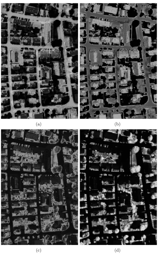
Figure 3.1: An example area from the data set. (a) Ortho photo. (b) DSM. (c) Reference data with class labels: impervious surfaces (white), building (blue), low vegetation (cyan), high vegetation (green), car (yellow).

point cloud data that were acquired by an airborne laser scanner [75]. The digital surface model (DSM) data, where height information of each pixel in the infrared images is stored, are provided as well. In the data set, there are two different types of DSMs that were generated using two different methods. The ones in the first group were generated from the original ortho photo images by dense matching using the Match-T software [76]. The DSMs in the second ground were generated by interpolating the point cloud with a grid width of 25 cm. Although its resolution is lower, we use the DSMs that were generated from the point clouds because they are more accurate. Since the Vaihingen area is huge, it is hard to process the raw infrared and DSM data. For this reason, the whole area has been divided into 33 tiles by the data set providers. Among these 33 tiles, only 16 of them have ground-truth. In addition, DSMs for 6 out of 16 regions are not usable. As a result, we use only area 1, 3, 5, 7, 11, 15, 29, 30, 34 and 37. In the data set there are 6 different classes; impervious surfaces (road), building, low vegetation (grass), high vegetation (tree), car and background. Only a few tiles have background objects. Infrared ortho photo image, DSM and ground-truth for area 3 can be seen in Figure 3.1.

(32)

3.2 Overview

We propose a method that is able to detect the classes in the ISPRS Vaihingen data set in a mostly unsupervised way by using spatial, spectral and height infor-mation of each pixel. Although there are 5 major classes and a background class in the ground-truth, we detect 4 of the classes; impervious surfaces, building, low vegetation, and high vegetation. The reason why our system is not able to detect cars is that the DSMs and infrared ortho photo images have been taken on different dates. For this reason, position of some of the cars in the 3 band images and the DSMs do not match.

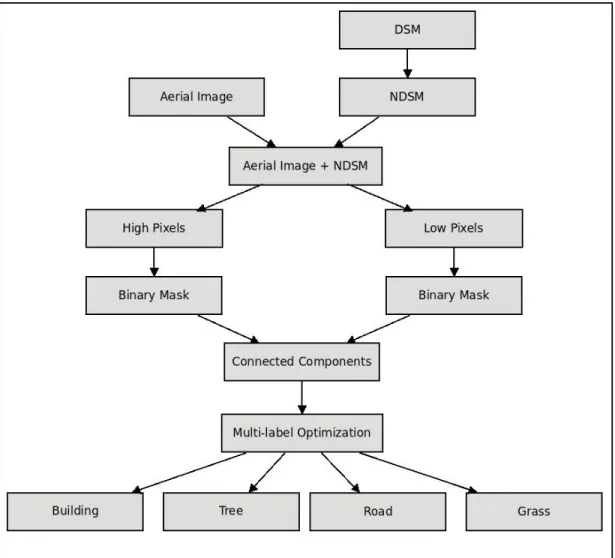
We begin with grouping the pixels in the data set as high and low by thresh-olding the DSMs according to height. We then extract binary masks for the high and low pixels, and find the connected components in these masks. The high pix-els constitute buildings and trees, whereas the low ones consist of roads and grass areas. However, at the end of this thresholding step, a small portion of the pixels can be classified incorrectly; high pixels may contain grass and road, and low pixels may have building and tree. We use two different graph cut procedures to detect classes in all of the connected components. The first procedure separates buildings from trees in each component in the high binary mask, and roads from grass in each component in the binary mask for the low pixels using the max-flow/min-cut algorithm described in [12, 13]. The flowchart of this framework can be found in Figure 3.2. In the second graph cut procedure, instead of run-ning max-flow/min-cut procedure in each connected component of the high and low binary masks separately, we apply the multi-label optimization [14, 15, 16] to each connected component in order to detect all of the classes directly. The flowchart of the proposed method that is based on the multi-label optimization can be found in Figure 3.3. Max-flow/min-cut algorithm provides an optimal solution [13] but multi-label optimization does not always guarantee an optimal solution [15].

(33)

Figure 3.2: Flowchart of the proposed method that is based max-flow/min-cut.

3.3 Preprocessing

In the preprocessing step, we generate binary masks for the high and low pixels by thresholding each DSM data and find the connected components in both of the masks. We use four different methods in order to divide the pixels in the DSMs as high and low. These are gray-scale reconstruction based on geodesic dilation, progressive morphological filtering, area opening and opening. Among these four methods, the progressive morphological filtering finds the high and low pixels directly. Others take a DSM as an input and generate another data, containing height information of the bare earth without objects on it. The resulting data are called the digital surface model (DTM). After generating the DTM, we subtract it from the DSM in order to generate the normalized digital surface model (NDSM),

(34)

Figure 3.3: Flowchart of the proposed method that is based on multi-label opti-mization.

which is another data that contains relative height information of each pixel above the estimated ground. We finally group the pixels as high and low by thresholding the NDSMs.

3.3.1 Grayscale Reconstruction Based on Geodesic

Dila-tion

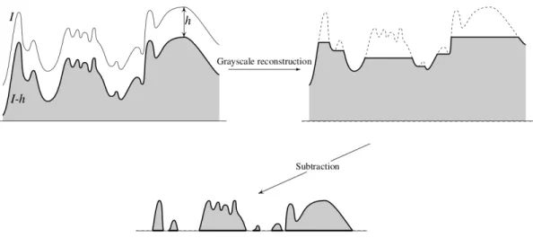
Gray-scale reconstruction takes two input gray-scale images with the same size. These images are called mask and marker. The marker image must be below the

(35)

mask image. In this algorithm, the marker image is dilated as long as it remains below the mask image. In other words, the mask image limits dilation of the marker image.

The marker and mask images are denoted by J and I respectively, and the structuring element is denoted by B. The gray-scale dilation of J and the struc-turing element B is

δ(J ) = J ⊕ B (3.1)

where ⊕ denotes the gray-scale dilation.

The geodesic dilation of J limited by I and dilated by the structuring element B sized 1 is

δ_I1(J ) = (J ⊕ B) ∧ I. (3.2)

Gray-scale reconstruction is obtained by applying the geodesic dilation succes-sively n times until the marker image fits under the mask image as

δn_I(J ) = δ_I1(J ) ◦ δ1_I(J ) ◦ . . . ◦ δ1_I(J )

| {z }

n times

. (3.3)

The DSM data corresponds to I in the equations above. When we apply the gray-scale reconstruction method to a DSM data, the resulting reconstructed image corresponds to DTM. More information about the gray-scale reconstruction and geodesic dilation can be found in [77], and applications of these algorithms to the DSM data can be found in [1].

The gray-scale reconstruction procedure is illustrated in Figure 3.4.

3.3.2 Progressive Morphological Filtering

The progressive morphological filtering algorithm [2] applies the morphological opening operation to the given DSM progressively. It first opens the DSM with an initial structuring element. After that, the opened image is substracted from the given DSM. Among the pixels in the resulting data obtained at the end of the substraction operation, the ones which are higher than the predefined threshold

(36)

Figure 3.4: Flowchart of the Gray-scale Reconstruction. Top-left image: I is the mask image (DSM), I-h corresponds to J, which is the marker image, Top-right image: reconstructed image (DTM), bottom image: difference between the DSM and DTM (NDSM). This figure was taken from [1].

value are labeled as non-ground whereas the others are labeled as ground. In the subsequent iterations, size of the structuring element is increased according to

wk= 2kb + 1 (3.4)

where wk is the size of the current structuring element, k is the iteration number

and b is the size of the structuring element. In addition to this, height threshold is also increased in each iteration as

dhT ,k=          dh0, if wk≤ 3 s(wk− wk−1) + dh0, if wk> 3 dhmax, if dhT,k > dhmax (3.5)

where dhT ,k is the current threshold, dh0 is the initial height threshold, dhmax is

the maximum height threshold and s is the slope of the area.

At the end of this algorithm, pixels of the given DSM image are labeled as ground and non-ground.

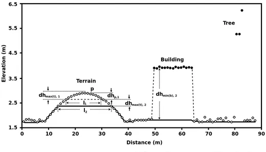
An illustration for the progressive morphological filtering algorithm can be found in Figure 3.5. As it can be seen from the Figure 3.5 that the height

(37)

Figure 3.5: Illustration for the progressive morphological filtering algorithm. I1

and I2 are sizes of the structuring elements, dhmax(t),1and dhmax(t),2 are the height

thresholds in the first and second iterations, and dhp,1 is difference between the

height of the pixel P in the original DSM image and the height of the same pixel in the opened image at the end of the first iteration. This figure was taken from [2].

difference of the pixel P in the DSM and opened image is smaller than the height threshold. For this reason, this pixel is labeled as ground. On the other hand, the height difference of a pixel, which belongs to the building in the DSM and opened image, is bigger than the height threshold. Therefore, it is labeled as non-ground.

3.3.3 Area Opening

In the binary area opening method, connected components are found in a binary image and the ones having an area smaller than the given threshold values are removed. The binary area opening method later has been extended to gray-scale area opening [78], where the given image I is decomposed into several gray-scale images by defining different gray levels and area opening of the image I is the

(38)

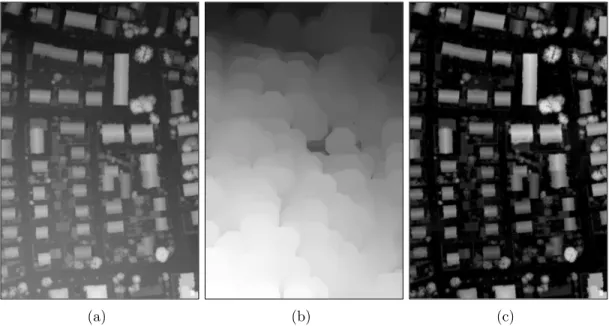
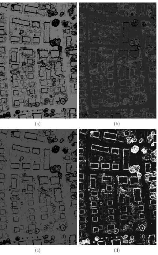
(a) (b) (c)

Figure 3.6: Illustration of NDSM generation using area opening. (a) DSM, (b) DTM obtained by using area opening, (c) NDSM generated by subtracting DTM from DSM. Each image in the figure has been normalized between 0-255 for better visualization.

supremum of the gray-scale images that are smaller than I and having larger area than the area threshold.

3.3.4 Opening

In order to generate DTMs from DSMs, we apply gray-scale morphological open-ing method successively. The openopen-ing operation starts with openopen-ing the input image by the structuring element whose shape is a disk with a radius of 3. In each iteration radius of the structuring element is increased according to

rcurrent = 2rpreviousk + 1 (3.6)

where k is the iteration number.

In the first iterations, since a small structuring element is used, the objects with a small width such as traffic lamps and small bushes are removed. As the size of the structuring element increases, the algorithm starts removing larger

(39)

(a) (b) (c)

Figure 3.7: Illustration of DSM generation using opening. (a) DSM, (b) DTM obtained by using opening, (c) NDSM generated by subtracting DTM from DSM. For the sake of visualization purposes, each image in this figure is normalized between 0 and 255.

objects. In the last iterations, the method removes the big buildings.

We separate the data set as high and low pixels using these four methods with different settings. To understand which method separates the best, we consider trees and building as one (high), roads and grass areas as another class (low), and calculate an accuracy for each method. Among these four methods classical gray-scale opening works the best. For this reason, in our experiments we use this method.

3.3.5 Generation of the Connected Components

After dividing the data set as high and low pixels, we extract binary masks for the separated pixels and find connected components in these masks. The main reason why we do not use the whole images is the issue of computational complexity. Since building very large graphs for the graph-cut procedures require extensive computational power, it is not feasible to use the images directly. Hence, we run

(40)

the graph-cut method in each component that is much more smaller than the whole image.

Example binary masks and their corresponding connected components can be found in Figure 3.8.

3.4 Features

We use several features that are based on spectral and height information. The features are explained in great detail in Sections 3.4.1 and 3.4.2.

3.4.1 Spectral Features

The first feature that is related to spectral information is color, which is self-explanatory.

The second feature in this category is normalized difference vegetation index (NDVI), which is one of the most common features in remote sensing applications because it is a very distinctive feature for the healthy vegetation. One condition to extract this feature is that the image must have infrared and red color bands. Intrinsically, the healthy vegetation reflects a large portion of the infrared light but absorbs most of the red light. However, for any other objects this situation does not apply.

NDVI is calculated as

N DV I = N IR − RED

N IR + RED (3.7)

where NIR is the Near Infrared band. The values that NDVI can take range from -1 to 1.

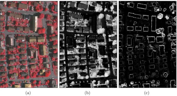
An example infrared image and the corresponding NDVI map can be seen in Figure 3.9.

(41)

(a) (b)

(c) (d)

Figure 3.8: Example binary masks, and their connected components. (a) Mask for the high pixels, (b) Mask for the low pixels, (c) Connected components of the high mask, (d) Connected components of the low mask.

(42)

As can be seen from Figure 3.9, the pixels belonging to trees and grass have very high NDVI value than the others.

3.4.2 Height Features

The features falling into this group is just the relative height information, which is stored in the DSMs, and irregularity that needs detailed explanation.

The pixels belonging to buildings, roads and grass mostly belong to planar shapes, whereas the ones belonging to trees have irregular shapes. For this reason, irregularity is a potentially distinctive feature to separate trees from the other classes.

Although the DSM is two dimensional data, since height information of each pixel is available in the DSMs, they can be considered as if they are three dimen-sional data. We slide a 7 × 7 pixel window on the DSM data. Using the x, y coordinates and the height information of the pixels in the window, we calculate a 3 × 3 covariance matrix. From this covariance matrix, we find the smallest eigenvalue. The resulting value is assigned as the irregularity value of the pixel that lies in the middle of the window. By repeating this operation, we find the irregularity value of each pixel in the DSM image. Since the the pixels belonging to roads, buildings and grass are parts of planar shapes, their the smallest eigen-values are very close to zero. On the other hand, the smallest eigenvalue of the pixels belonging to trees are larger.

An example area and corresponding irregularity map can be seen in Figure 3.9. As it can be observed from the figure that irregularity value of the pixels belonging to trees are high, whereas most of the pixels that belong to the other classes have lower irregularity. However, there are some pixels causing problems as well. The pixels, which lie at the borders of buildings have a relatively high value for the irregularity because when calculating the smallest eigenvalue for these pixels, some of the pixels falling into the sliding window are on the building, whereas the others are on the ground. A similar problem also applies to some of

(43)

(a) (b) (c)

Figure 3.9: An example infrared ortho photo image and its corresponding feature intensity maps. (a) Infrared image, (b) NDVI map, (c) Irregularity map.

the trees. Some small vegetation patches such as bushes have planar shapes. As a result, the pixels belonging to these sort of vegetation have small irregularity values.

These problems are solved by the graph cut procedures explained below.

3.5 Graph Cuts

3.5.1 Max-flow/Min-cut Procedure

We detect buildings and trees by applying the max-flow/min-cut framework de-scribed in [12, 13] to the connected components of the binary mask for the high pixels. We repeat the same operation in order to separate roads from grass in each connected component of the binary mask for the low pixels.

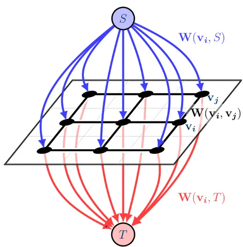
In this graph cut framework, each node in the graph corresponds to a pixel in the connected component. There are also two specially designed terminal nodes

(44)

Figure 3.10: An example graph model for the max-flow/min-cut procedure. named source S and sink T . In our problem, the source corresponds to one class of interest (e.g., building or grass) and the sink corresponds to another (e.g., tree or road). All of the nodes in the graph are connected to both the source and the sink nodes, and all of the neighboring nodes are connected to each other with weighted edges. The weight between two neighboring nodes is the cost of cutting the edge between these nodes. The weight between a node corresponding to a pixel in the image and a terminal node, which represents a class of interest is the cost of assigning the node to the terminal node. The goal of the cut procedure is to assign each of the nodes to one and only one of the terminal nodes by cutting some edges. An example graph model can be seen in Figure 3.10.

Let C be the class set and f be a particular feature value of a pixel. The probability of assigning the pixel to class c using the feature value f is calculated

(45)

as

p(c | f ) = _Pp(f | c) · p(c)

c∈C

p(f | c) · p(c) (3.8)

where p(c | f ) is the posterior probability and p(f | c) is the class-conditional probability distribution function (pdf) for feature f . p(c) is the prior probability for class c. The classes are assumed to be equally probable in the rest of the thesis.

In order to calculate the posterior probabilities, probability distributions that model the likelihood of each pixel in each class for each feature need to be es-timated. We estimate the probability distributions of all of the classes for the NDVI feature by Gaussian mixture models with four components and for the irregularity feature by exponential functions. For the height feature, we estimate the distributions of road, grass and tree by exponential functions, and distribu-tion of building by a Gaussian mixture model. The models are selected based on visual inspection.

Histograms for the irregularity, height and NDVI values, and the fitted models can be seen in Figures 3.11, 3.12 and 3.13. The pixel posterior probability map and the posterior probability distribution of each class for each feature can be seen in Figures 3.15, 3.16 and 3.17 and 3.18, respectively.

Let V correspond to the set containing all pixels and N be the set consisting of all pixel pairs in a connected component. We define the vector A = (A1, . . . , A|V |)

as the binary vector whose elements Av are the labels for the pixels.

In order for the max-flow/min-cut framework to detect the classes in each con-nected component, we define a cost function. The max-flow/min-cut procedure cuts some of the edges for minimizing the cost function. At the end of the cut operation, each node in the graph is assigned to either the source or the sink ter-minal node. The cost function to separate buildings from trees in the connected components for the high masks is defined as

E(A) = λ1· RNDVI(A) + λ2· RIrregularity(A)

| {z } Data Cost + λ3· BSpatial(A) | {z } Smoothness Cost (3.9)

(46)

where

Ri(A) = X

v∈V

Ri_v(Av), i ∈ {NDVI, Irregularity} (3.10)

accumulates the individual penalties for assigning pixel v to a particular class Av

based on the NDVI and the irregularity features. For the smoothness cost in (3.9), we use two different definitions. We run our experiments for these two smoothness cost definitions, and compare and discuss the results that are obtained using both definitions. The first definition for the BSpatial_{(A) term is}

Bspatial(A) = X

{u,v}∈N

δAu6=Av (3.11)

which penalizes the cases where neighboring pixel pairs have different class labels (δAu6=Av = 1 if Au 6= Av, and 0 otherwise).

The second definition is

BSpatial(A) = X {u,v}∈N Bu,v· δAu6=Av (3.12) where Bu,v = p (D (u, v)) (3.13) and D(u, v) = kC(u) − C(v)k . (3.14)

The C (·) in (3.14) stands for color information of the given pixel.

Both (3.11) and (3.12) enforce spatial regularization, where neighboring pixels have similar labels as much as possible. The only difference between these two definitions is that rather than assigning a constant to the cost of cutting the edge between two neighboring pixels as described in (3.11), we give a higher weight to the edge between two neighboring pixels if their color is similar to each other, and give a lower weight if their color difference is high in (3.12). To accomplish this task, we estimate the probability distribution that models the likelihood of color distance between two neighboring pixels. Histogram of the distances between all pairs of neighboring pixels and the fitted exponential model can be seen in Figure 3.14.

(47)

(a) (b)

(c) (d)

Figure 3.11: Histograms and the estimated probability distributions of each class for the NDVI feature. NDVI values are modeled using Gaussian mixture models with 4 components. (a) road, (b) building, (c) grass and (d) tree.

R_vi(Av) is defined according to the classes of interest. Since the cut procedure

minimizes a cost function by removing (i.e., cutting) some of the edges, the weight of a pixel that is connected to the terminal node that corresponds to the correct class should be low as the penalty for assigning that pixel to the correct class should introduce a low cost. We use the posterior probabilities to determine the costs. The posterior probabilities are calculated using (3.8), where C = {building, high veg.}.

In particular for the separation of buildings from high vegetation the Ri v(Av)

(48)

(a) (b)

(c) (d)

Figure 3.12: Histograms and the estimated probability distributions of each class for the irregularity feature. The irregularity values are modeled using Exponential models. (a) road, (b) building, (c) grass and (d) tree.

is defined as

R_vNDVI(Av = building) = −p(building | n), (3.15)

R_vNDVI(Av = high veg.) = −p(high veg. | n), (3.16)

R_vIrregularity(Av = building) = −p(building | ir), (3.17)

R_vIrregularity(Av = high veg.) = −p(high veg. | ir). (3.18)

where n is the NDVI and ir is the irregularity value of pixel (node) v. λ1, λ2 and

λ3 in (3.9) determine the relative importance of each term.

We define another cost function to discriminate road and grass in the connected components of the low binary mask. However, as it can easily be observed from

(49)

(a) (b)

(c) (d)

Figure 3.13: Histograms and the estimated probability distributions of each class for the height feature. Height values of roads, grass and trees are modeled using Exponential models, and height values of buildings are modeled by a Gaussian mixture model with 4 components. (a) road, (b) building, (c) grass and (d) tree. Figure 3.9 that the irregularity is not a convenient feature to separate roads from grass because height variance of the points belonging to either of these two classes is low. Therefore, in this part of the method, we do not use the irregularity feature in the cost function. The cost function is

E(A) = λ1· RNDVI(A)

| {z } Data Cost + λ2· Bspatial(A) | {z } Smoothness Cost . (3.19)

For the smoothness cost in (3.19), we follow the same steps we do in (3.11) and (3.12). The posterior probabilities are calculated using (3.8), where C =

(50)

Figure 3.14: Histogram and the estimated probability distribution for the dis-tances between two neighboring pixels. The disdis-tances are modeled using Expo-nential fit.

{road, low veg.}. The terms in the data cost are defined as

RNDVI_v (Av = road) = −p(road | n), (3.20)

RNDVI_v (Av = low veg.) = −p(low veg. | n). (3.21)

Finally, we merge the classification maps coming from the low and high pixels to get only one classification map.

3.5.2 Multi-label Optimization Procedure

The graph model for the multi-label optimization procedure [14, 15, 16] is quite similar to the one for the max-flow/min-cut framework. The main difference is that instead of two terminal nodes as in the max-flow/min-cut procedure, there can be any number of terminal nodes in this framework. In our case, there are four terminal nodes because we have four different classes. Another important point is that although there are four terminal nodes, the cut procedure does not have to assign at least one pixel to each of the classes. If none of the pixels fits to a class, the cut procedure may not assign any pixels to that class.

The irregularity is a distinctive feature to detect trees, and NDVI is a con-venient feature to separate healthy vegetation (tress and grass) from roads and

(51)

(a) (b)

(c) (d)

Figure 3.15: Posterior probability map of each class for the ndvi feature. (a) road, (b) building, (c) grass and (d) tree.

(52)

(a) (b)

(c) (d)

Figure 3.16: Posterior probability map of each class for the irregularity feature. (a) road, (b) building, (c) grass and (d) tree.

(53)

(a) (b)

(c) (d)

Figure 3.17: Posterior probability map of each class for the height feature. (a) road, (b) building, (c) grass and (d) tree.

(54)

(a)

(b)

(c)

Figure 3.18: Posterior probability distributions of each class for (a) NDVI, (b) irregularity, (c) height.

Object detection using optical and lidar data fusion with graph-cuts

OBJECT DETECTION USING OPTICAL

AND LIDAR DATA FUSION WITH

GRAPH-CUTS

a thesis submitted to

the graduate school of engineering and science

of bilkent university

in partial fulfillment of the requirements for

the degree of

master of science

in

computer engineering

By

Onur Ta¸sar

March 2017

ABSTRACT

OBJECT DETECTION USING OPTICAL AND LIDAR

DATA FUSION WITH GRAPH-CUTS

¨

OZET

C

¸ ˙IZG ˙E KES˙IT ˙ILE OPT˙IK VE LIDAR VER˙I VER˙I

F ¨

UZYONU KULLANARAK NESNE TESP˙IT˙I

Acknowledgement

Contents

List of Figures

List of Tables

Chapter 1

Introduction

1.1

Motivation and Problem Definition

1.2

Contribution

1.3

Outline

Chapter 2

Related Works

Chapter 3

Methodology

3.1

Data set

3.2

Overview

3.3

Preprocessing

3.3.1

Grayscale Reconstruction Based on Geodesic

Dila-tion

3.3.2

Progressive Morphological Filtering

3.3.3

Area Opening

3.3.4

Opening

3.3.5

Generation of the Connected Components

3.4

Features

3.4.1

Spectral Features

3.4.2

Height Features

3.5

Graph Cuts

3.5.1

Max-flow/Min-cut Procedure

3.5.2

Multi-label Optimization Procedure