A novel CAD algorithm for the analysis of printed geometries

(1)

М Ш Ш Ш : Ш 1 1 1 І Й М У Ш 5 ? · · ΓΓ^ν:ίΐ·>

A DsSSSFïTAri і>Сй;·^

SuB¿!,4sTTs0 т с TAîI S»?=iAiñT$^;jS:rT о ? SLSST^’CAI. Aí>íD £LEGT?s£riMÄ

^i<Z;· TH¿ ?)-í3TíT'iT£ OF

ENGi^ÆEB^S

¿ i S SCfEíjOS O? B'Li<£r-iT ü?'-i!VSRo-Tv·' !■."■<' i' Í-A.L FOLr3i-j_-feâ£îFr OF Тн-Е F!i^!;0'î?ïSîsï3>:TS DOCTOR OF PHsLOSCAHY ííOJ/áñ ß ч 1Ö Q -V.._l ’ТО ..’ L 'tj/ iJr J

(2)

A DISSERTATION

SUBMITTED TO THE DEPARTMENT OF ELECTRICAL AND ELECTRONICS ENGINEERING

AND THE INSTITUTE OF ENGINEERING AND SCIENCE OF BILKENT UNIVERSITY

IN PARTIAL FULFILLMENT OF THE REQUIREMENTS FOR THE DEGREE OF

DOCTOR OF PHILOSOPHY

By

Noyan Kinayman

May 1997

(3)

те

■К56 -İ93^

(4)

M. I. Aksun, Ph. D. (Supervisor)

I certify that I have read this thesis and that in my opinion it is fully adequate, in scope and in quality, as a dissertation for the degree of Doctor of Philosophy.

Abdullah Atalar, Ph. D.

(5)

Giilbin Dural, Ph. D.

Approved for the Institute of Engineering and Science:

A

Mehmet Baray,

Director of Institute of Engineering and Science V. P h . a /

(6)

(7)

Abstract

A NOVEL CAD ALGORITHM FOR THE ANALYSIS OF

PRINTED GEOMETRIES

Noyan K in aym an

Ph. D. in Electrical and Electronics Engineering

Supervisor:

Assoc. Prof. M. I. Aksım

May 1997

An efficient and accurate computer aided design (CAD) software for the electromagnetic simulation of passive microwave components, fabricated in planar stratified media, is developed in this work. The numerical technique employed in this software is based on the spatial-domain method of moments (M oM ) in conjunction with the closed-form Green’s functions. Since the computational efficiency is a major issue in CAD softwares, the spatial-domain MoM is significantly improved in this respect with the use of the closed-form Green’s functions and closed-form expressions for the MoM matrix entries. Vertical metalizations in the form of via holes and shorting pins, which are the indispensable parts of the most microwave circuits, are also modeled very efficiently and incorporated into this formulation. The resulting approach is applied to some realistic microwave circuits and planar antennas, with and without vertical metalizations, to validate the formulation. It is also demonstrated that the formulation developed in this work can be efficiently used with an optimization algorithm for design purposes. The results obtained from the formulation proposed in this work are compared to those obtained from a commercial electromagnetic analysis software.

Keywords: CAD, Printed structures. Full-wave EM analysis, Planarly layered media. Green’s functions. Method o f moments

(8)

DÜZLEMSEL GEOMETRİLERİN ANALİZİ İÇİN YENİ BİR

CAD ALGORİTMASI

Noyan Kınayman

Elektrik ve Elektronik Mühendisliği Doktora

Tez Yöneticisi:

Doçent Doktor M. I. Aksım

Mayıs 1997

Bu çalışmada, düzlemsel çok katmanlı ortamlardaki pasif mikrodalga devrelerinin elektromanyetik simulasyonu için hızlı ve hassas bir bilgisayar destekli tasarım yazılımı geliştirilmiştir. Bu yazılımda kullanılan sayısal tekniğin temelini kapalı formdaki Green’s fonksiyonları ile birlikte kullanılan uzay boyutu moment metodu oluşturmaktadır. Analiz hızı, bilgisayar destekli tasarım yazılımlarında önemli bir özellik olduğu için, uzay boyutundaki moment metodu kapalı formdaki Green’s fonksiyonları ve matris elemanları kullanılarak oldukça iyileştirilmiştir. Kısa devre bağlantıları ve katmanlar arası geçişi sağlayan bağlantılar şeklindeki düşey metalizasyonlar da verimli bir şekilde modellenmiş ve formulasyona dahil edilmiştir. Elde edilen yazılım, forrnulasyonu doğrulamak amacıyla, düşey metalizasyon da içeren bazı gerçekçi mikrodalga devrelerine ve düzlemsel antenlere uygulanmıştır. Bu çalışmada geliştirilen formulasyonun bir optimizasyon algoritması ile verimli olarak kullanılabileceği de gösterilmiştir. Bu çalışmada önerilen formulasyondan elde edilen sonuçlar, bu alanda kullanılan ticari bir programın sonuçları ile karşılaştırılrmştır.

Anahtar Bilgisayar destekli tasarım, Tam-dalga EM analizi. Düzlemsel çok Sözcükler: katmanlı ortam, Green’s fonksiyonları. Moment metodu

(9)

Acknowledgment

I would like to express my deepest gratitude to Assoc. Prof. M. I. Aksun for his supervision and encouragement in all steps of the development of this work.

My special thanks go to my colleague Lale .Alatan for inspiring discussions on many topics in this thesis, and Aydın Alatan for his invaluable helps during my study.

And my dear friends, I was not able to list the names of all of you here, please forgive me about that. Müşerref, Şükrü, and Feyza, it was your continuous encouragement which gave me a great moral support.

I am grateful to the members of my rock band for sharing many pleasant moments with me. Making music has always been a kind of “discharge” for me.

Finally, my sincere thanks go to my family for their love and patience throughout my graduate study. It is their unhesitating self-sacrifice which has enabled me to achieve my goals in my life.

(10)

Acknowledgment

Contents i

List of Figures iv

List of Tables viii

1 Introduction 1

1.1 A Brief Review of the Analysis Methods of Printed Structures . . 2

2 Green’s Functions in Planarly Layered Media 5 2.1 Green’s Functions in Spectral Domain 6 2.1.1 Horizontal electric dipole (H E D )... 9

2.1.2 Vertical electric dipole ( V E D ) ... 11

2.1..3 Green’s functions for electric and magnetic dipoles... 12

2.2 Closed-form Green’s Functions in Spatial D o m a in ... 14

2..3 C o n c lu s io n s ... 18

3 Field Analysis in Planarly Layered Media 19 3.1 MPIE Formulation in Planarly Layered M e d ia ... 20

3.1.1 Difficulties and S olu tion s... 24

3.1.2 Singularities Encountered in the Application of MoM . . . 29

3.2 The Method of De-embedding of the Port Discontinuities... 31

(11)

3.3.1 Microstrip Patch A n t e n n a ... 3-5

3.3.2 Microstrip C o rn e r... 38

3.3.3 Proximity Coupled Microstrip Patch A n t e n n a ... 42

3.3.4 Microstrip Patch Antenna with Parasitic Elements 45 3.3.5 Four-pole Elliptic Band-pass F i l t e r ... 45

3.3.6 3 dB 90° Hybrid C ou p ler... 46

3.3.7 Coupled-line Band-pass F i l t e r ... 51

3.3.8 Interdigital MIC C apacitor... 51

3.3.9 Short-circuited Microstrip Line 56 3.3.10 Air B r id g e ... 57

3.3.11 Short-circuited Microstrip Patch Antenna .58 3.3.12 Square-spiral MIC I n d u c t o r ... 61

3.4 C o n clu sio n s... 64

4 Methods for Improving the Analysis Time 65 4.1 Evaluation of the MoM Matrix E n t r ie s ... 68

4.1.1 Numerical E x a m p le s ... 69 4.2 Interpolating Frequency D a t a ... 78 4.2.1 Numerical E x a m p le s ... 80 4.3 C o n clu sio n s... 83 5 Optimization 84 5.1 Genetic A lg orith m s... 85 5.2 Numerical E x a m p le s ... 87 5.3 C o n clu sio n s... 92 6 Conclusions 93 A Explicit Forms of the Green’s Functions 95 A .l The Green’s function G l ... 95

A .2 The Green’s function ... 96

A.3 The Green’s function Gf^. 96

(12)

B . l Evaluation of 6'J * ... 9S

B.2 Evaluation of 99

B.3 Evaluation of G\ * ...100

B.4 Evaluation of {Tzm·, G'^, * Jzn')...101

B.5 Evaluation of the other t e r m s ... 101

C Generalized Pencil of Function Algorithm 102 D Method of Moments 108 D . l Variational Interpretation ... 109

E Series Acceleration Methods Used in EM 112 E. l The Transformation M e t h o d s ...113

E.1.1 Euler’s Transformation... 114

E.1.2 Shanks’ Transformation ...114

E.1.3 Method of Averages ... 116

E.1.4 The Θ A lg orith m ... 117

E.1.5 The Chebyshev-Toeplitz A lg o r it h m ...117

E .l.6 The Poisson Transform ation...118

E .l.7 Ewald’s Transformation ...119

E .l.8 Rummer’s Transform ation... 120

E .l.9 Method of E x p o n e n tia ls... 121

E.2 Results and D iscu ssion ... 122

E.2.1 Integration Involving Bessel Functions ...122

E.2.2 Free-Space Periodic Green’s F u n c t io n s ...126

E.2.3 Quasi-Dynamic Green’s F u n c t io n ... 129

E.3 C on clu sion ... 130

Vita 143

(13)

List of Figures

2.1 A general source placed in a planarly stratified medium. 7 2.2 The path used in exponential approximation... 16 3.1 A typical multilayer printed geometry... 20 3.2 Basis functions used for horizontal and vertical connections in the

MoM solution... 22 3.3 Cross-section of a planar circuit with a vertical connection showing

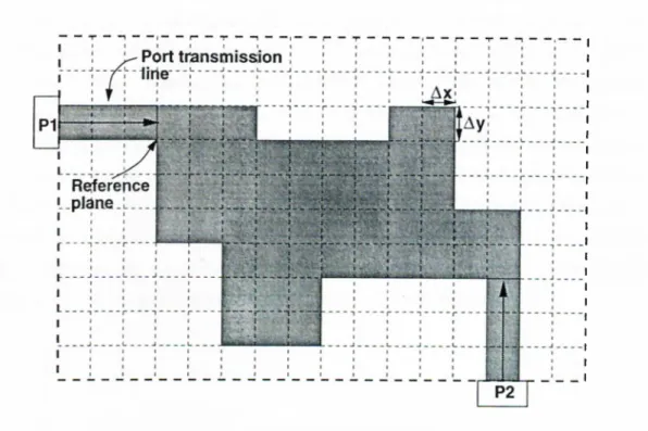
the discontinuous basis functions... 30 3.4 Meaning of £g// for ^ microstrip transmission tine... .34 3.-5 Typical gridding which is used in the simulation software... 3-5 3.6 Geometry of a patch antenna... 36 3.7 r,„ of the patch antenna shown in Fig. 3.6. Frequency increases

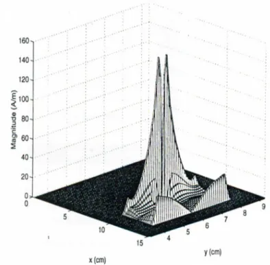
in the clock-wise direction (/siari=2200 MHz, /s/op=2400 MHz). 37 3.8 a:-directed current density of the patch antenna shown in Fig. 3.6

at / =2300 MHz... 38 3.9 i/-directed current density of the patch antenna shown in Fig. 3.6

at / =2300 MHz... 39 3.10 Geometry of a microstrip corner... 40 3.11 Magnitude of Su of the microstrip corner shown in Fig. 3.10. . . . 40 3.12 Phase of Sn of the microstrip corner shown in Fig. 3.10... 41 3.13 Equivalent lumped circuit model of the microstrip corner shown

in Fig. 3.10... 42 3.14 Geometry of a proximity coupled patch antenna... 43

(14)

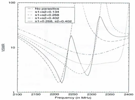
3.16 Ecjuivalent lumped circuit model of the proximity coupled patch antenna shown in Fig. 3.14... 44 3.17 Geometry of the microstrip patch antenna with parasitics... 46 3.18 Input V SW R of the microstrip patch antenna with parasitics

shown in Fig. 3.17... 47 3.19 Geometry of a band-pass filter... 48 3.20 Magnitude of of the band-pass filter shown in Fig. 3.19 for

different s values... 48 3.21 Magnitudes of and 5'2i of the band-pass filter shown in Fig. 3.19

for s=0.175 cm ... 49 3.22 Geometry of a hybrid coupler... 49 3.23 Magnitudes of 5i3 and Su of the hybrid coupler shown in Fig. 3.22. 50 3.24 Phases of S

13

and of the hybrid coupler shown in Fig. 3.22. . . 50 3.25 Geometry of a multilayer band-pass filter... 51 3.26 Magnitudes of Su and S'21 of the band-pass filter shown in Fig. 3.25. 52 3.27 Phases of and ^2 1 of the band-pass filter shown in Fig. 3.25. . 52

3.28 Geometry of an interdigital MIC capacitor... 53 3.29 Magnitudes of and S'21 of the MIC capacitor shown in Fig. 3.28. 54

3.30 Phases of S'!! and S'21 of the MIC capacitor shown in Fig. 3.28. . . 54

3.31 Magnitudes of S'!! and S

21

of the MIC capacitor shown in Fig. 3.28. 55 3.32 Equivalent lumped circuit model of the interdigital capacitor

shown in Fig. 3.28... 56 3.33 Geometry of a short-circuited microstrip line... 57 3.34 Current distribution on the microstrip line shown in Fig. 3.33 with

a single shorting pin... 58 3.35 Current distribution on the microstrip line shown in shown in

Fig. 3.33 with three shorting pins... 59 3.36 Geometry of an air bridge... 59

(15)

3.37 Magnitude of of the air bridge shown in Fig. 3.36... 60 3.38 Phase of 5 u of the air bridge shown in Fig. 3.36. 60 3.39 Geometry of a shorted microstrip patch antenna... 61 3.40 Resonant frequency of the patch antenna, shown in Fig. 3.39, vs.

shorting pin location... 62 3.41 Geometry of a MIC square-spiral inductor... 63 3.42 Magnitude of the input impedance of the MIC inductor shown in

Fig. 3.41... 63 4.1 Flow-chart of the hybrid inethod for evaluating the MoM matrix

entries... 70 4.2 Matrix fill-time vs. auxiliary parameter s for the patch antenna. . 71 4.3 Magnitude of the input impedance of the patch antenna for

different values of s ... 72 4.4 Phase of input impedance of the patch antenna for different values

of s ... 73 4.-5 Mean matrix fill-time vs. auxiliary parameter s for the interdigital

capacitor... 74 4.6 Magnitudes of ¿'ll and ^2i of the interdigital capacitor for different

values of s ... 75 4.7 Phases of ¿"n and ¿ 2 1 of the interdigital capacitor for different

values of s ... 76 4.8 Magnitudes of ¿'ll and ¿'21 of the interdigital capacitor for different

number of sampling points... 76 4.9 Magnitudes of Sn and ^ 2 1 of the interdigital capacitor for different

number of sampling points and interpolation scheme... 77 4.10 Flow-chart of the frequency interpolation... 79 4.11 Magnitude of ¿'ll of the patch antenna shown in Fig. 3.6 (exact:21

points, interpolated:7 points)... 80 4.12 Phase of ¿'ll of the patch antenna shown in Fig. 3.6 (exact:21

points, interpolated:7 points)... 81

(16)

4.14 Phases of Su and S

21

of the band-pass filter shown in Fig. 3.25

(exact:41 points, interpolated: 15 points)... 82

5.1 Flowchart of a typical genetic algorithm used in the optimization process... 86

5.2 Geometry of the the proximity coupled microstrip antenna with tuning stub... 88

5.3 Fin of the the proximity coupled microstrip antenna shown in Fig. 5.2 before and after optimization... 90

5.4 Matrix solve times during the optimization process on a SUN SPARC 20 workstation for each analysis... 91

5.5 Matrix fill times during the optimization process on a SUN SPARC 20 workstation for each analysis... 91

E .l Relative errors for the integral given in Eq. ( E .3 9 ) ...124

E.2 Relative errors for the integral given in Eq. ( E .3 9 ) ... 124

E.3 Relative errors for the integral given in Eq. ( E .3 5 ) ... 125

E.4 CPU times for different number of evaluation points for the integral given in Eq. ( E . 3 5 ) ...126

E.5 Relative errors for the summation given in Eq. ( E .4 0 ) ...127

E.8 CPU times for different acceleration methods applied to Eq. (E.19) 129 E.9 Relative errors for the summation given in Eq. ( E .4 3 ) ... 130

(17)

List of Tables

3.1 Equivalent lumped circuit values for the microstrip corner shown in Fig. 3.10... 42 3.2 Equivalent lumped circuit values for the proximity coupled patch

antenna shown in Fig. 3.14... 45 3.3 Equivalent lumped circuit values for the interdigital capacitor

shown in Fig. 3.28... 56 4.1 CPU times in terms of seconds consumed in the analysis of some

typical geometries on a SUN SPARC 20 workstation... 67 4.2 CPU times in terms of seconds consumed in the analysis of some

typical geometries with adaptive s parameter selection on a SUN SP.ARC 20 workstation... 77 5.1 Parameters of the genetic algorithm used in the optimization. 89 E.l Summary of the transformations used in the exam ples... 123

(18)

Introduction

The history of microwave printed circuits begins with the invention of flat-strip coaxial transmission lines by V. H. Rumsey and H. W. Jamieson to use in an antenna system and power division network during World War II [1]. Later, Hewlett Packard Co. developed the “slotted line” which was a commercial application of a planar coaxial system. Then, it was shown by Robert M. Barrett that the planar circuits could be also used to build passive microwave components like filters, directional couplers, and hybrids [1]. .\fter the realization of the potential of the printed circuits, R&D facilities have been concentrated in this field to explore the possible application areas. Some of the research centers worked on this field were Tufts University, the .\irborne Instruments Laboratory (Strip Line), the Polytechnic Institute of Brooklyn, Sanders Associates (Tri- Plate). and Federal Communications Research Laboratories (Micro-Strip) [1]. Because the printed circuits are rugged, easy to produce and reproducible, and because they have low cross-section and weight which make them useful in air borne applications, they have quickly gained a lot of interest and have been used in many applications in places of their waveguide and coaxial line counterparts.

The advent of monolithic microwave integrated circuits (.MMIC) has increased the importance of printed structures in planarly layered media. Thus, development of a rigorous and efficient technique to characterize such structures has become an important issue in computational electromagnetics. Once the

(19)

analysis is performed with the use of a rigorous full-wave method, the lumped circuit model of the passive structure can be extracted to use in a circuit simulation program with active devices. In addition, interactions between the passive circuits, like coupling between array elements in a microstrip antenna array, can also be investigated more rigorously.

CHAPTER 1. INTRODUCTION

2

1.1 A Brief Review of the Analysis Methods of

Printed Structures

There have been a flurry of activities in the area of computational electromag netics to develop computationally efficient and accurate numerical techniques for modeling and simulating the electrical performances of printed circuits. Basicly, there are two approaches in the characterization of such structures: approximate but numerically efficient methods, like quasi-static methods [2-4] and accurate but computationally expensive methods such as the method of moments (Moi\I) [5,6], the finite element method (FEM) [7] and the finite-difference time domain (FDTD ) method [8].

The FDTD method is formulated by discretizing the Maxwell’s ecpiations both in the space and time domains. One of the advantages of the FDTD method is that the frequency response of the circuit can be extracted through a band of frequency by applying a narrow Gaussian pulse excitation in the time domain. The FEM is a general numerical technique to find approximate solutions to the boundary value problems. In the FEM, the entire volume is divided into sub volumes in which the unknown function is represented by simple interpolating functions. Then, a set of algebraic equations is obtained by applying the Rayleigh- Ritz procedure. Common advantages of the above mentioned methods are that they are quite general and versatile and that the resulting matrix equations are sparse yielding an efficient memory and CPU time requirements for solving this system of linear equations. However, both methods have difficulties when they are applied to open geometries, like radiating structures, because they require

(20)

discretization or segmentation of the whole volume of interest. In this case, artificial absorbing boundaries should be introduced to satisfy the radiating condition. On the other hand, the MoM is applied to an integral equation that accounts for the geometry, so the problem domain is reduced to regions where the surface or volume current densities can be defined. The advantage of this technique, as compared to the FEM and the FDTD, is the reduced number of unknowns and its suitability for planar geometries. However, the major disadvantage is that the MoM matri.x entries are double or triple integrals of complex functions.

Since the MoM is used as the main numerical technique throughout this work, it would be instructive to give a brief introduction of the technique as applied to planar printed geometries in electromagnetics. The formulation of the MoM starts with writing an integral equation describing the problem, which could be electric field integral equation (EFIE), magnetic field integral equation (.MFIE) or mixed potential integral equation (MPIE). The formulations of EFIE and MFIE involve the Green’s functions of the electric and magnetic fields as their kernels, respectively, while the MPIE uses the Green’s functions of the scalar and vector potentials. Since the Green’s functions of the electric and magnetic fields are more singular than those of the scalar and vector potentials, the MPIE formulation has recently become more popular in the application of the MoM to the characterization of planar printed geometries [9-12]. Therefore, the MPIE formulation is employed in this work and its solution is obtained via the MoM. The MoM can be applied either in the spectral dornciin or in the spatial domain. The spectral domain version is applied to the spectral domain representation of the EFIE while the spatial domain version is applied to the MPIE. In this thesis, the spatial-domain MoM is employed because of the aforementioned advantage of the MPIE. .Although the Green’s functions used in the spectral-domain representation of the EFIE can be e.xpressed in closed forms for planar printed geometries, the MoM matrix entries become double integrals of complex functions over infinite domain, which requires the use of computationally expensive numerical integration algorithms. On the other hand, the MoM matrix

(21)

CHAPTER 1. INTRODUCTION

entries for the spatial-domain MoM are double integrals over finite domains, but the integrands are in terms of the spatial-domain Green’s functions of the potentials, which are expressed as the Hankel transforms of the corresponding spectral-domain Green’s functions [13,14]. Since the Hankel transforms of the spectral-domain Green’s functions are oscillatory and slow convergent in nature, the use of the spatial-domain MoM was not popular until the recent introduction of an efficient algorithm to approximate the spatial-domain Green’s functions in closed forms [15,16]. This closed-form approximation of the spatial-domain Green’s functions not only improves the calculation of the Green’s functions, but also results in the MoM matrix entries that can be evaluated analytically [17]. Therefore, the computational efficiency of the spatial-domain MoM in the solution of the MPIE has been significantly improved without sacrificing the accuracy in the results.

In this thesis, the MPIE in the spatial-domain employing the closed-form Green’s functions is used to find the current distribution on the conductors which are immersed in a planarly layered medium. The organization of this thesis is as follows: In Chapter 2, the spectral- and spatial-domain Green’s functions for planarly stratified media are introduced. Then, in Chapter 3, a general MPIE formulation for planarly stratified media is presented using the closed- form spatial-domain Green's functions, and some numerical examples are given. Chapter 4 discusses some approaches that are used to improve the total solution time of the circuits. Then in Chapter 5, a brief introduction is provided for the optimization of printed circuits with genetic algorithms. Firuilly the conclusions are given in Chapter 6.

(22)

Green’s Functions in Planarly

Layered Media

For a planarly layered medium, the spatial-domain Green’s functions are obtained from the spectral-domain Green’s functions via the Hankel transformation, in which the spectral-domain Green’s functions are known in closed forms for layered media [18,19]. This transformation, also known as .Sommerfeld integral, contains oscillatory integrand over an infinite domain whose evaluation is computationally very expensive [20], hence the apparent disadvantage of the spatial-domain MoM formulation.

Recently it was demonstrated that the computational burden in the calculation of the spatial-domain Green’s functions can be circumvented by approximating the spectral-domain Green’s functions in terms of complex exponentials, whose Hankel transforms can be analytically obtained via the Sommerfeld identity [1-5]. Hence, the spatial-domain Green’s functions for the vector and scalar potentials can be cast into, so called closed forms, which are finite sums of complex images. In this approach the crucial step is the numerical implementation of the exponential approximation, which can be performed by using Prony’s techniques [21] or techniques based on the pencil of functions [22,23]. The original derivation of the closed-form Green’s functions, as proposed by Chow et. al. [15], employed the original Prony method and was limited in

(23)

use to thick and single layer structures, which was due to inadequacy of the original Prony method. This problem was eliminated by employing the least squares Prony method [24], and then the approximation was further improved by using the generalized pencil of functions method (GPO F) [19], which is less noise sensitive and more robust as compared to the Prony methods (see -Appendix C). However, the algorithm for the exponential approximation was still computationally expensive, because Prony’s methods and the GPOF method require uniform sampling of the function to be approximated along the range of approximation. This, in turn, makes it necessary to take a large number of samples for functions with local oscillations and fast variations, like spectral- domain Green’s functions in general, rendering the algorithm computationally expensive and not robust. Recently, a two-level approach that recjuires piecewise uniform sampling has been introduced to eliminate this problem, and is demonstrated to be much more efficient and robust [25]. Hence, the spatial- domain closed-form Green’s functions can be employed efficiently in the solution of MPfE for planar, multilayer geometries. There are also other approaches where an asymptotic closed-form Green’s functions are obtained [26,27], however it should be noted that the closed-form Green’s functions derived by the method given in this thesis are valid in all spatial regions.

In Section 2.1, the spectral-domain Green’s functions for planarly stratified media are given. Then, Section 2.2 describes the method of obtaining the closed- form spatial-domain Green’s functions. .And finally, conclusions are given in Section 2.3.

2.1 Green’s Functions in Spectral Domain

CHAPTER 2. GREEN’S FUNCTIONS IN PLANARLY LAYERED MEDIA

6

Consider a general source placed in a planarly stratified medium which is shown in Fig. 2.1. ft is assumed that all layers extend to infinity in the horizontal plane, and, the thickness and the relative permittivity of ¿-th layer are denoted by d, and Cr., respectively. Note that the origin of the coordinate axis is placed at the bottom of the source layer, and the time convention of has been adopted

(24)

through the formulation.

1+1

^i+m * observation point (z)

z=z m »observation point (z) z=z 2=Z, • source point (z’) _z=0 _X z=z l-n z=z

Figure 2.1: A general source placed in a planarly stratified medium.

In a planarly hiyered medium, the electrical properties of the structure change only in one direction, e.g., in the z direction. For that reason, the vector wave equations need not be solved in their full forms. In fact, in the source-free case, the vector wave equations can be reduced to two scalar equations representing T E and T M waves which are decoupled from each other [18].

In the MPIE formulation, the Green's functions of both vector and scalar potentials are used. It is known that for a horizontal dipole, two components of the vector potential are reciuired to satisfy the boundary conditions [28,29]. Traditionally, the z-component is selected in addition to the component which is in the same direction with the dipole. The Green’s function, in this case, will have the following form:

G

ta

—

{^xx

-f"

yy') G

XX “h

-

_jx

G

;

x

-f-

-^yG2y

“t

” Gzz

(2.1)

(25)

CHAPTER 2. GREEN’S EUNCTIONS IN PLANARLY LAYERED MEDIA

8

Hertzian dipole can be derived from the vector potential via [28]

· Ga = — Y 'G ,

(2.2)

However, since the scalar potential depends on the chosen form of the magnetic vector potential in a layered medium, it is not unique. That is, the scalar potential associated with a vertical dipole is different from the scalar potential of a horizontal dipole when the medium is stratified. Therefore, a single scalar potential G', satisfying (2.2) does not, in general, exist if the traditional form of the vector Green’s function Ga, given in (2.1). is employed.

To find the spectral-domain Green’s functions, the field components of a Hertzian dipole in the a direction, which is placed in a homogeneous medium, are written as / - V V \ (2.3) E (r) = - i ^ ^ p + — H (r) = V X a a ll-- j k r -l/rr (2.4)

from which the T M and T E field components of the dipole can be derived easily. Since the dipole is in a layered medium, the spherical wave behavior in (2.3) and (2.-1) must be modified. This is achieved by expanding the spherical wave terms in terms of plane waves using the Weyl identity

, - j k r — jr^r J ■ /.QQ roo

V wTT J — OoJ — OQ cI)J\yy L· (2.5)

where i·^ + ky + = Lq. Then reflections from the planar boundaries of the stratified medium, can be easily accounted for the field expressions. Note that since the medium is translationally invariant in the xp plane, the phase matching condition requires that kj; and ky are the same in all layers.

The spectral-domain Green’s functions are first derived in the source layer by considering the direct wave, and the reflected waves from the boundaries, as shown in the next sections. Then, the field in any other layer can be obtained from the field expression of the source layer.

(26)

2.1.1 Horizontal electric dipole (HED)

Derivation of the spectral-domain Green’s functions for an HED starts with writing Ez {TM~) and H, {TE^) components of the fields in the source layer. So, E, and IT are first written in a homogeneous medium as

j l l E, = H, = 4Tru;t dz dx r II d (2.6) (2.7) 4TT dy r

Then, the spherical wave terms are expressed as an integral summation of the plane waves propagating in all directions using the WTiyl identity

IIIL E, = — ---- / / ^TT^UJSi J —ooJ — oo H -~ 87t2 / oo roo

/

dkx clky ky -cc>J—oo ^-jk:cJ:-jkyy-jk=^ |~| (

2

.

8

) (2.9)

Since these expressions are valid in a homogeneous medium, the fields in a layered medium are obtained by considering the reflected waves from the boundaries as follows: II E. = / CO /*00 --XjJ—OO II

11

/■^o /-X)/- oo /• X) ^-JksX-jkyy y ^y---j--- ^TE (

2

.

10

) (2.11) where Fte = " e-Aniz-z') ^ ^ > , - j k , , ( z ' - z ) ^ ^ ( j e -3k . ^ ( z - z ‘ ) Ftm = < r < c > (2.12a) (2.126) < r' e-Az,{z-z') ^ ^ _e-^k.,(z'-z) ^ B lC k-(z-z') A·.-,

Note that the origin is at the bottom of the source layer in this derivation (see Fig. 2.1). The down-going wave in the source layer is the conseciuence of the

(2.13a)

(27)

CHAPTER 2. GREEN’S FUNCTIONS IN PLANARLY LAYERED MEDIAIO

reflection of the up-going wave at 2 = cL, similarly, the up-going wave is the

consequence of the reflection of the down-going wave at ~ = 0. Hence.

+ (2.14)

+ (2.15)

where Rtm is the generalized reflection coefficient at the boundaries [18]. By solving (2.1-1) and (2.1.5) simultaneously, the unknown coefficients and are found as B-TM e — Ktm tiTu e ' Dl = iTM 1 _ p-j2k,.d, „ — i'

2

kz z' I D*|*+1 ~ Rtm ^ I Rtm Rtm ® .A (2.16) (2.17) 1 _ D'-*+l ¿»■•-l^-i2fc.-.di 1 eiTM ^TM ^

.Since the same approach is used to find the other coefficients,

A\

and

C^,

their derivations are not given here for the sake of brevity. To derive the vector Green's functions, one can proceed as follows:

A^ = -Mi J H,dy

II /f·^CO rco ^~JkxZ: jktjij / dk^ dky--- --- Fte -CO./-CO A-v (2 .IS) => = j

2

k,,L· -b (2.19)

A,

= Mi

_{j H^dy = ¡.li j ^}

- H . + j u e - E .IT , ■ ^ C dy ¡.till /■'»

S

t

T^

J -

_oo

J-Ml kx (

2

.

20

) dkx dky e | k Q··^ — _ Stt^ . / —o o J —rXJ + + (2.21)

and for the scalar Green’s function.

(f>d

= “ “

V · A

1 i dAx dAC

(28)

4 >d

=

d

,

**dx'*"**

^ G l

_X

=

2 cikl \

A:-,

,

A·-.

(2.23) L. (2.24)

2.1.2 Vertical electric dipole (VED)

The derivation of the spectral-domain Green’s functions for a VED is similar to the approach used for HED, therefore it will be briefly given here. As a first step. E^ and / / . components of the fields due to a VED are written as follows:

E. = jllu fl

4'irk'^ k^ + dz'^

j

r = 0

(2.25) (2.26)

Then, by using the Weyl identity, (2.25) is expanded as

E. = - Ilu>l.l / oo roc> ( Jc^ / dk, dky — - k,, -ooJ-oc· \ k.. (2.27) J -ooJ -oc·

Next, the field expression in a layered medium is obtained by considering the reflected waves as II E. = where Et.v = < -

r r

dk,dkyk,e~^^^^-^^^^FTM i J—ooJ — oo (2.28) (2.29a) - j k . ^ ( z - z ' ) ^ Q y k x , ( z - z ' ) , ^ _(2.296)

Using the boundary conditions at the interface of the layers, the unknown coefficients A® and obtained as before. To derive the vector Green’s function, one can proceed as follows:

1 r ^

(29)

CHAPTER 2. GREEN’S FUNCTIONS IN PLANARLY LAYERED MEDIA12

f

= ^ 8 ^ 7r r dK dky — ooJ—oo ^ ^ 1 Frxf

^ G i = + . 4 : , e - ^ · ^ · - - · (2. 31)

aud for the scalar Green’s function,

V ·

A I d A .

4>d —

h = (2-33)

^ G \ = + (2.34)

where the unknown coefficients are obtained from the boundary conditions as before.

2.1.3 Green’s functions for electric and magnetic dipoles

In summary, the spectral-domain Green’s functions in the source layer for different kind of sources and orientations, are obtained by using the described method as follows [19]:

2

jL·, f'A _

■ W .

, - j k . , \ z - z ' \ ^ j A . - . . , ^ { A l

+

B l)

^

{D l - C l) (2.35) GV = 1 + 2j€iL·, i ^ f c t - m ,-ik.Az-z^ K K (2.37) = CPr = ■2jL·,

2

jL·, 1 yk.,U-z'\ ^ ^ ^ + B l') e '‘ ‘ .(-= 'l + ( / ) ” -

c;;‘)

1,2 D m i 1.2 Am - j k . , \ z - z ' \ ^ ') + 2ji-iik,, 1,2/^m 1,2 Dm - l ^ z . ^ h - i k , . (z-z> )

_(2.40)

(30)

GV-G f; 6'!"‘ /i.

2

jL·, 1

2

j ^ikzi e.·

2

jL·, 1 e-Nz,\z-z'\ ^ ^ ^ - j k . , \ z - z ' \ 4 ^ ^ -^ ·^ ·--. ^ A;,. (2.41) (2.42) (2.43) (2.44)

where the superscript /1 and F denote the electric and magnetic vector potentials, respectively, and qm denote the electric and magnetic scalar potentials, respectively. The coefficients, C^’^ , and D l’^ are the functions of the generalized reflection coefficients and are given [IS, 19] as

Лe,m h _ p^î+1 jkfTEyTM Be,m _ 5*\î + lIV MiTM, TE Ce,rn L jje^ m yi e,m B e , m ^ e , m D e , m T M J E - ^t e j m’^h T M J E i,i — l T M J EMi _ p i . i+1 \ j T E — ^TMJE^^^i __ p i . i - 1 j irlWiJE — ^TMJE^^^i e -t-- 2 j k , ^ { d , -t-- z ' ) _ D i ,i - 1 . - 2 j k , ^ d , ^ ^TMJE^ __ 1 rTM, TE ^ - ¿ j k z , [ d , - z ' ) , f,-2jkz^d, e -t- nrM.TE^ — f.-‘^Nz,z' I D‘.‘ + l f,-'

2

'jkz^d, _ f > - ‘^ N z , ( d , - z ’ ) I D ‘ . ‘ - l - 2jkz, d, where MiTE, TM ^J+hj 1 _ R‘ -‘ + l p-Jkz,2d, dJ + I-J I o i J - l -jk - 2dj ^TE.TM I ^TE.T\C ^ - 1 TE, TM (2.45) (2.46) (2.47) (2.4S) (2.49) (2..50) (2.51) (2..52) (2..53) (2.54) 1 D . . C > i5 -1 2dj

Here R and R are the Fresnel and generalized reflection coefficients [18] for which the subscripts T E and T M represent the polarization of the wave, and the superscripts show the layer numbers. The subscripts h and v represent the orientation of the source, horizontal and vertical, respectively, while the superscripts e and m denote the type of the source, electric and magnetic, respectively. It should be noted that the Green’s functions for y-oriented dipoles

(31)

can be obtained simply by setting G ff/ k y = G f//k^, and

Q'U.m

^ y

GT-VVlien the observation layer is different from the source layer, the Green’s functions are modified by using the appropriate boundary conditions and following iterative expressions [18]:

^7 = ^7+1 4 = 1 -1 -(2.55) (2.56) where A~ and Aj~ are the amplitudes of the down- and up-going waves, respectively, and T is the transmission coefficient. So, the field expressions in any layer can be obtained iteratively starting from the source layer.

2.2 Closed-form Green’s Functions in Spatial

Domain

The spatial-domain Green’s functions are obtained from the spectral-domain counterparts through an integral transformation, called the Hankel transform or the Sommerfeld integral in electromagnetics [13]. This transformation is given as

G = 7 /

47T Js i p

d k ,k,H ^ T \ K p)G {kp) (2.57)

where G and G are the Green’s functions in the spatial and spectral domains, respectively, is the Hankel function of the second kind and S I P is the Sommerfeld integration path. The spectral-domain Green’s function, which is the integrand of the Sommerfeld integral given in Eq. (2.57), contains branch-point and pole singularities. The branch-point singularities correspond to radiating modes in the outermost layers, whereas, the pole singularities correspond to guided modes in the dielectric layers.

In principle, there are two ways for evaluating the Sommerfeld integral when the exact analytical integration is not possible: i.) Asymptotic methods like

(32)

the method of stationary phase and the method of steepest descent [18], and Ü.) numerical integration methods [1-1]. Although the asymptotic methods give better physical understanding of the integral itself, they must be re-formulated for different geometries, hence they are not suitable to use in a CAD software. On the other hand, the numerical integration of the Sommerfeld integral is computationally e.xpensive procedure because the integrand is an oscillatory complex function with the singularities mentioned above, and because the limits of integration extent to infinity. As a conclusion, the evaluation of the Sommerfeld integral with the aforementioned methods is not suitable for a CAD algorithm [20,25].

To eliminate the numerical integration of the Sommerfeld integral, the spectral-domain Green’s functions are approximated by complex exponentials, whose Hankel transforms can be evaluated analytically, thus the spatial-domain Green’s functions can be written in closed-forms [15,25]. This procedure was first proposed by Chow et.al. [15] for a horizontal electric dipole over a thick substrate and extended to a geometry with a substrate and superstrate with arbitrary thickness by Aksun and Mittra [2-1].

The original approach of getting the closed-form Green’s functions in the spatial domain requires some trial-and-error iterations for deciding the approximation parameters, like the number of exponentials, the number of sampling points and the maximum range of the approximation. Moreover, the c[uasi-dynamic images and the surface wave poles need to be found and extracted from the Green’s function prior to the approximation in order to ease the difficulties in the algorithm. However, with the introduction of the two-level approach, which is robust and very efficient, these difficulties are eliminated, and hence the method becomes very suitable for C.AD implementation [25]. It should be noted that the sampling of the spectral-domain Green’s functions should be performed along the SIP or along a path legitimately deformed from the SIP, details of which can be found in [15,25]. In this thesis, we have employed a deformed path from the SIP as depicted in Fig. 2.2, consisting of three connected paths denoted as 6api, Cap

2

and Capz·, respectively, and described by the following

(33)

parametric equations:

For Cap3 ■ — ~jLi [Foi + To

2

+ t\ For Ca,p

2

■ = ~ jk i [Toi + t] For C.pi : L A·,

0 < i < To3 0 < t < 7’o2 0 < t < T o i (2.58) (2..59) (2.60) where t is the running variable sampled uniformly on the corresponding ranges, Toi, To

2

·, and Toz- This approach is named hereafter as three-level approach, which is an extension of the two-level approach introduced recently [25], so its details are not included in this thesis. Because the spectral-domain Green’s functions might have fast variations locally, and because the GPOF method requires uniform sampling along the range of approximation, the use of multi level approach prevents taking thousands of samples. However, it is not necessary to use the three-level approach for smooth functions, for which one may use the two-level or one-level approach, simply by setting T03 to zero or T

02

and To

3

to

zero, respectively.

kp plane

— I---1--- *—

►-ko k,

P m a x i P m a x 2 P m a x 3

Figure 2.2: The path used in exponential approximation.

The exponential approximation process begins with sampling the function to be approximated, and then the algorithm for exponential approximation is employed for the sampled values of the function. In other words, one needs to know the values of the function at the points of samples, which requires fixing the parameters, like 2 and z' in Eqs. (2.35)-(2.44). After having sampled the spectral-

(34)

GPOF method is used to obtain the exponential approximation of the function, which results in an approximation as follows:

N3

( 7 S

1 ( N

1

N

2

(2.61)

n=l n = l

Once the spectral-domain Green’s functions are represented as the sum of complex exponentials, each exponential term in (2.61) can be transformed to the spatial domain via the Sommerfeld identity

^-jkr

=

1 /

2¿j JsiP / Jsi dk, ■ [kpp)" ' k,

yielding the following Green’s function expression in the spatial domain

(2.62) ^1 Q-jkirin G = ain— --- h ^ o,2n ^2 g-jk,r2n ^3 Q-jkirin n=l n = l r-2n + ^2 n= 1 f'Zn (2.63)

where = y / ~ ¿im '^2n = - ¿2u, r.3„ = yjp'^ - 6§„, and p = ^j,·- + cirid, a „ ’s and 6„ ’s are complex numbers in general.

The extraction of the surface wave poles and the quasi-dynamic images helps to the exponential approximation technique, as stated before, by rendering the Green’s functions in the spectral domain well-behaved and rapidly converging functions. However, since the contribution of the surface wave poles is small for geometries on a thin substrate, and it is not possible to find the quasi dynamic images for multilayer planar structures analytically except for some simple cases, the spatial-domain Green’s functions are obtained for a multilayer medium without extracting the surface wave poles and quasi-dynamic images in order to obtain a general-purpose algorithm.

(35)

CHAPTER 2. GREEN’S EUNCTIONS IN PLANARLY LAYERED MEDIAIS

2.3 Conclusions

The use of the closed-form Green’s functions has eliminated the numerical integration of the Sommerfeld integrals improving the computational efficiency of the spatial-domain MoM for planar geometries in multilayer media.

The original algorithm developed for obtaining the closed-form spatial-domain Green’s functions has the disadvantage of choosing the proper appro.ximation parameters for each different geometry. Moreover, the extraction of the surface wave poles and quasi-dynarnic images may not be possible or efficient for multilayer geometries when the original version of the approach is employed. The new approach based on a three-level approximation is developed to overcome these difficulties and to make the use of the closed-form Green’s functions attractive for those developing the EM software as well as for researchers in the field.

(36)

Field Analysis in Planarly

Layered Media

Formulation of the spatial-domain MoM for the analysis of printed geometries begins with writing the MPIE in terms of the Green’s functions of vector and scalar potentials in a multilayer medium. Then, the integral equation is discretized by expanding the unknown current densities in terms of known basis functions and by applying the boundary conditions in integral sense, which is called as the testing procedure in the MoM. This formulation has the advantage of employing the MPIE, whose kernel shows a weak surface integrable singularity while the EFIE involves stronger singularity, but it recjuires the Green’s functions in the spatial domain. The spatial-domain Green's functions are obtained in closed form by using the technique presented in Chapter 2. .After .solving the

linear system obtained by the application of the .MoM, the current distribution on the conductors is found. For more information about the MoM, one can refer to .Appendix E.

In Section 3.1. a general formulation of the problem is given. Section 3.2 presents the de-embedding algorithm which is used in the S-pararneter calculation of the printed circuits. Then, in Section 3.3, some numerical examples are given.

Finally, the conclusions are presented in Section 3.4.

(37)

3.1 MPIE Formulation in Planarly Layered

Media

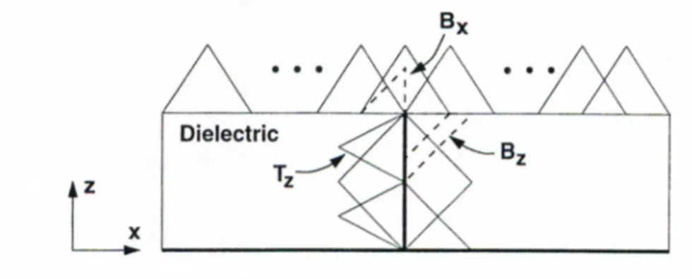
Considei·, for the sake of illustration, a general microstrip structure in a multilayer environment as shown in Fig. 3.1. It is assumed that all layers and the ground plane extend to infinity in the horizontal plane, and the conductors are lossless and infinitesimally thin. The thickness and the permittivity of ¿-th layer are denoted by di and respectively. .Although the geometry depicted in Fig. 3.1

CHAPTER 3. FIELD ANALYSIS IN PLANARLY LAYERED MEDIA

₂₀

Figure 3.1: A typical multilayer printed geometry.

shows only one vertical metalization, the formulation given here can be applied to printed geometries which contain multiple vertical metalizations.

The tangential components of the electric field on the plane of the patch and on the vertical strips can be written in terms of the surface current density J, and the associated Green’s functions of the vector and scalar potentials as follows:

1 d

E.V = - j wG],^ * Jx

(38)

E , = - r w G f y j + J - | - V ■ J) jiu d y 1 d (3.2) Ez — j wCt.j. * Jx jwCt. * Jy jw C “^, ^ J, -\- -— i^CP' + V · J) (3.3) J W U Z '

where * denotes convolution and G'4 = The term G'd represents the i-directed vector potential at r due to a j-i-directed electric dipole of unit strength located at r', while G'’"- represents the scalar potential by a unit point charge associated with an electric dipole. Since the traditional form of the Green’s functions are employed in the formulation, the Green’s function of the scalar potential is not unique for horizontal and vertical electric dipoles as stated previously. Hence, the term involving the Green’s function of the scalar potential, which is common in Ecjs. (3.1)-(3.3), can be e.xplicitly written as

G'^‘ * V · J GJ' * ^ + Gl'· * ^ + GV- * ^

ux ^ ay ^ oz (3.4)

where GtJ'- G·'^-j and Gl'- denote the Green’s functions of the scalar potential for a horizontal and vertical electric dipoles, respectively.

do solve for the surface current density J via the MoM. J is expressed as a linear combination of suitable sub-domain basis functions;

771 71 771 n Jz{x,lj,z) =

y,.)

(3.5) (3.6) (3.7)

where and are the basis functions with the unknown coefficients and defined at (mn)-th position on the subdivided horizontal conductor and at (/)-th position on the subdivided vertical conductor. In this thesis, rooftop functions are chosen as the basis functions to represent x-, y- , and z-components of the current density, as shown in Fig. 3.2. The sources are modeled as current filaments, therefore it is suitable to use half-rooftop basis functions at the source terminals, as well as at the sink terminals where the shorting pins or via holes are terminated in the ground plane. At the

(39)

22

P^igure 3.2: Basis functions used for horizontal and vertical connections in the MoM solution.

intersections of the vertical and horizontal conductors, half-rooftop and saw tooth basis functions are employed on the vertical and the horizontal conductors, respectively, whose amplitudes are related to satisfy the conservation of charges. Fig. 3.2.

Following the substitution of Eqs. (3.o)-(3.7) into Eqs. (3.1)-(3.3), the boundary conditions for the tangential electric fields are implemented in integral sense through the testing procedure of the MoM, for which the field e.xpressions multiplied by some testing functions j^V) are integrated on the conductors and are set to zero. This leads to a matrix equation for the unknown

(40)

coefTicients of the basis functions as

7 7 7

^xx ^xy ^XZ ^yX Zyy Zyz Zru Z

2

:

■ Ix ' ' Vx '

ly = Vy

L

(3.8)

where Zs denote the mutual impedances between the testing and basis functions, and V^s represent the excitation voltages due to the current source(s). The matrix entries corresponding to the horizontal and the vertical rnetalizations can be written explicitly as follows:

Q Q { m n ) ' ( :k dx z . * dx Yxy --7 — ^yx --7 _ ^yy — Z._x = 2:.. = J _ / rp(m'n') j u \ " ' dx ^ / rp(m'n') ______ Ix d Q Q (m n) * — - — dy dy QQ(m n) CP'- * — ^ dx - j u , G i . i L Q<U ^ ---- y----" dy d B i‘^ - j u {tP , G i » ^ ( P /\ ^ ^ / rp(^m'n') ^ j u ’ dx GV * QB(mn) dx G'^' * dz dB i‘^ QB(mn) CP:· ---- y----dy z , . ^ / rp[m'n') ^ J ^ Y ^ ' dy Gl' * dB'i^ d l (3.9) (3.10) (3.11) (3.12) (3.13) (3.14) (3.15) (3.16) (3.17)

where < , > and * denote inner product and convolution operators, respectively, and they are defined as follows:

(41)

f ( x , y) * g{x, y) =

JJ

d x 'd y 'fix - x ’ , y - y') ■ g[x\ y') (3.19) The entries of the array V have the same form except the basis function, which is a half-rooftop function with unit amplitude to model the current source, therefore they are not given here. After evaluation of the inner product terms and substituting into Eq. (3.8), the current densities on the conductors are obtained by solving the matrix equation. Then, the scattering parameters are extracted from the current distribution.

The use of the closed-form Green's functions in conjunction with the MoM has been demonstrated to improve the computational efficiency of the MoM when applied to simple geometries like those consisting of only horizontal conductors. After having improved the computational efficiency and robustness of the derivation of the closed-form Green’s functions, the natural step towards the goal of developing an accurate and efficient EM simulator is to study this approach for general geometries. .A preliminary study shows that the application of the MoM in conjunction with the closed-form Green’s functions to a geometry with vertical metalizcition is not as straightforward as its applications to only horizontal geometries, i.e., there are some difficulties in cases of vertical metalizations [30].

3.1.1 Difficulties and Solutions

₂₄

The difficulties originate from the way the closed-form Green’s functions are derived, more specificly, from the exponential approximation of the spectral- domain Green’s functions. In Chapter 2, the representative form of the spectral- domain Green’s functions is given and it is stated that the parameters, c and z ', have to be fixed in order to be able to sample the function over the range of approximation. In other words, the exponential approximation is valid for only those fi.xed values of the parameters, so are the closed-form Green’s functions. For horizontal conductors, fixing 2 and z' does not pose a problem because the

conductors are situated on constant z-planes recjuiring the Green’s functions to be evaluated at these planes only. Therefore, one can fix these parameters prior

(42)

to the derivation of the closed-form Green’s functions, and use these Green’s functions for those values of the parameters only. However, the evaluations of the MoM matrix entries corresponding to the vertical metalizations reciuire the convolution integrals and the inner-product integrals given in Ecjs. (3.13)-(3.17), w’hich are to be integrated over z and/or Y. So, the closed-form Green’s functions, derived as described in Chapter 2, can not be used efficiently in the evaluation of such matrix entries.

This difficulty can be eliminated by recognizing that the amplitudes of the up- and down-going waves in the spectral-domain Green’s functions are the exponential functions of z' that can be factored out (see Appendix A). As an example, the spectral-domain Green’s function for the scalar potential due to a VED can be written as

1 Gl = + 2;k .e , SGi-f ^TM } (3.20)

after having substituted the amplitudes of the up- and down-going waves. Note that Rtm find MJ^^ are not functions of z and z', and their explicit expressions are given in Chapter 2. A brief study of Ec[. (3.20) shows that there are two approaches to overcome the difficulty: i.) application of the exponential approximation to each amplitude term, and ii.) performing the integration over z and z' analytically in the spectral domain, then applying the exponential approximation process. In the first approach, one needs to deal with each term in Ecp (3.20) separately; the first one is the direct term with unity amplitude, so no need for approximation, and the rest have amplitudes as functions of kp. In other words, the approximation of Gl in terms of complex exponentials with the exponents including z and z' explicitly requires to approximate only the amplitude functions of the four exponentials in Eq. (3.20). namely ,

Rt\\i^ A lf^ ^ a n d The cost of having z and z' explicitly in the approximation of a Green’s function is to apply the GPOF method three times more and is to use exponentials four times more as compared to approximating the same Green’s function as a whole. The second solution is based on the fact

(43)

that c and z' dependence of the spectral-domain Green’s functions is always in exponential form and analytically integrable over r and z' for most basis functions. Therefore, the integration over z and z\ which are due to the testing and convolution integrals along a vertical metalization, respectively, can be evaluated analytically if the spatial-domain Green's functions in the inner- product expressions are written as the inverse transforms of their spectral- domain representations. Then, the exponential approximation procedure is implemented on the resulting spectral-domain function. This approach eliminates the application of the exponential approximation for each term in the spectral- domain Green’s function. However, it requires the application of the e.xponential approximation as many times as the number of testing functions, or number of basis functions, or number of basis times testing functions on the vertical metalization for the inner-product terms involving c, or z' , or :: and z' integrations, respectively. Although the second approach seems to employ the exponential approximation algorithm more than the first one, it is more efficient for short vertical metalizations for which only a few basis functions are used. For one basis function on the vertical metalization which is usually sufhcient for a practical geometry, the number of exponential approximation in the second approach is less than that in the first approach, and moreover it requires less number of exponentials even for several basis functions. Also note that some of the commercial em simulation softwares, like em from SONNET, use only one basis function along a vertical metalization [31].

The first approach described above is quite straightforward, where one needs to write the spectral-domain Green’s functions in terms of exponentials of ; and z' with complex coefficients and to apply the GPOF method tor each complex coefficient. Therefore, there is no need to give further details for this approach. On the other hand, since the application of the second approach requires some work in the spectral-domain, it would be instructive to give the procedure and the details:

1. Write the spectral-domain Green's functions into the sum of exponentials of :: and z' with complex coefficients.

(44)

2. Express the spatial-domain Green’s functions in the MoM matrix entries as the inverse transforms of their spectral-domain representations using Eq. (2.57).

3. Evaluate the integrals over 2; and/or z' variables analytically.

4. Approximate the resultant expression by complex exponentials via the GPOF method.

5. Transform the whole expression into the spatial domain via the Sommerfeld identity Eq. (2.62), getting an auxiliary function which has the same form as Eq. (2.63).

6. Evaluate the remaining inner-product integrals analytically in the spatial domain.

The exponential approximation with the GPOF method in item 4, should be performed with care, because it has been obser\'ed that the functions obtained after evaluating 2 and z' integrals may contain peaks for intermediate values of

kp. Therefore, to capture such behaviors efficiently, the two-level approximation scheme is extended to three levels for these terms, as explained in Chapter 2. Hence, it is guaranteed that the spectral-domain auxiliary functions are approximated successfully. It should also be noted that addition of multiple vertical strips will not increase the computational cost of this technique, provided that all vertical strips employ the same number of basis functions. This is because the MoM matrix entries corresponding to the basis functions on a vertical strip are obtained as a function of p and because the domains of integrations along the vertical strips are the same. In other words, once the interaction between a basis and a testing functions on a vertical strip is calculated, the same expression can be used with a different value of p for the calculation of the reaction of the same basis function and a testing function (or vice versa) located on another vertical strip at a distance of p.

(45)

₂₈

term involving an integration on z —variable is considered:

(rf 1, G i * si""») =

I J d z d y T P i g , : )

■ jjd x 'd y 'a tix - x \ y - y\

Ij')

(3.21)

The first step of the procedure is to write the spectral-domain Green’s function G'}^ (2.36) in the form of Eq. (A .6), where r and z' dependencies are explicit. Then, the spatial-domain Green’s function Gd^ in Eq. (3.21) is replaced by the inverse transform of the spectral-domain Green's function Gj^^ (A.6). Hence, the inner-product term in Eq. (3.21) becomes

=

_{JJd zd yT P {y)T p iz)}

■

_JJdx'dy'

--)}

r t (:!.22)

where the separability of the basis functions is utilized, ::) = P y'^ z). After changing the order of integrations, the following au.xiliary function is defined and cast into closed form via the Sommerfeld identity:

e l =

/

_{d k ,k ,H P ix \f ,-f ,'\) 9 i!d !^}

J 4TT J s i P —J Px

- h ¡SIP

I /

‘*·

~

’ }(3.23)

where G P O F {·} designates the approximation process with complex exponentials via the GPOF method. Note that G^^ has a multiplicative term of —jkj;, which needs to be eliminated for being able to apply the GPOF method. This is the reason why Gf^ is divided by —jkj; and its effect is added in the spatial domain as a derivative with respect to xk Therefore, the argument of the G P O F {·} operator is approximated with complex exponentials without —jk^ term, resulting in the following inner product expression: