ANALYSIS OF PARALLEL ITERATIVE
GRAPH APPLICATIONS ON SHARED
MEMORY SYSTEMS
a thesis submitted to
the graduate school of engineering and science
of bilkent university
in partial fulfillment of the requirements for
the degree of
master of science
in
computer engineering
By
Funda Atik
January 2018
ANALYSIS OF PARALLEL ITERATIVE GRAPH APPLICATIONS ON SHARED MEMORY SYSTEMS
By Funda Atik January 2018
We certify that we have read this thesis and that in our opinion it is fully adequate, in scope and in quality, as a thesis for the degree of Master of Science.
¨
Ozcan ¨Ozt¨urk(Advisor)
U˘gur G¨ud¨ukbay
S¨uleyman Tosun
Approved for the Graduate School of Engineering and Science:
ABSTRACT
ANALYSIS OF PARALLEL ITERATIVE GRAPH
APPLICATIONS ON SHARED MEMORY SYSTEMS
Funda Atik
M.S. in Computer Engineering Advisor: ¨Ozcan ¨Ozt¨urk
January 2018
Graph analytics have come to prominence due to their wide applicability to many phenomena of real world such as social networks, protein-protein interactions, power grids, transportation networks, and other domains.
Despite the increase in computational capability of current systems, developing an effective graph algorithm is challenging due to the complexity and diversity of graphs. In order to process large graphs, there exist many frameworks adopting different design decisions. Nonetheless, there is no clear consensus among the frameworks on optimum design selections.
In this dissertation, we provide various parallel implementations of three rep-resentative iterative graph algorithms: Pagerank, Single-Source Shortest Path, and Breadth-First Search by considering different design decisions such as the order of computations, data access pattern, and work activation. We experi-mentally study the trade-offs between performance, scalability, work efficiency of each implementation on both real-world and synthetic graphs in order to guide developers in making effective choices while implementing graph applications.
Since graphs with billions of edges can fit in memory capacities of modern shared-memory systems, the applications are implemented on a shared-memory parallel/multicore machine. We also investigate the bottlenecks of each algorithm that may limit the performance of shared-memory platforms by considering the micro-architectural parameters.
Finally, we give a detailed road-map for choosing design points for efficient graph processing.
¨
OZET
ORTAK BELLEKL˙I S˙ISTEMLER ¨
UZER˙INDE C
¸ ALIS
¸AN
PARALEL TEKRARLAYAN C
¸ ˙IZGE
UYGULAMALARININ ANAL˙IZ˙I
Funda Atik
Bilgisayar M¨uhendisli˘gi, Y¨uksek Lisans Tez Danı¸smanı: ¨Ozcan ¨Ozt¨urk
Ocak 2018
C¸ izge analiz uygulamaları; sosyal a˘glar, proteinler arası etkile¸simler, g¨u¸c nakli ¸sebekeleri, ta¸sıma a˘gları gibi bir¸cok alana uygulanabilirlikleri sayesinde gittik¸ce ¨
onem kazanmı¸stır.
C¸ izge veri setlerinin karma¸sık ve ¸cok ¸ce¸sitli yapıda olması nedeniyle, g¨un¨um¨uz sistemlerinin sayısal i¸slem yapabilme kapasitesi artsa da etkili bir ¸cizge algorit-ması geli¸stirmek son derece zordur. B¨uy¨uk ¸cizge veri setlerini i¸slemek amacıyla ¨
onceden hazırlanmı¸s yapıların ve fonksiyonların bulundu˘gu farklı dizayn kararları alan bir¸cok ¸cer¸ceveler geli¸stirilmi¸stir. Fakat bu ¸cer¸ceveler arasında en iyi tasarım se¸cimlerinin nasıl olaca˘gı hakkında ortak bir karar yoktur.
Bu tezde; i¸slemlerin uygulanma sırası, veri eri¸sim bi¸cimleri ve i¸s aktivasyonu gibi farklı tasarım kararları g¨oz ¨on¨une alınarak, tekrarlayan ¸cizge uygulamalarına ¨
ornek te¸skil eden ¨u¸c algoritmanın ¸ce¸sitli paralel geli¸stirmeleri sunulmu¸stur. Bu ¨
u¸c algoritma ¸sunlardır: ”PageRank”, ”Tek Kaynaklı En Kısa Yollar” ve ”Sı˘g ¨
Oncelikli Arama”. Her bir uygulamanın, hem ger¸cek hem de sentetik ¸cizge veri setleri ¨uzerinde performans, ¨ol¸ceklenebilirlik ve i¸s verimi analizleri yapılarak bun-lar arasında nasıl bir denge kurulabilece˘gi deneysel olarak ara¸stırılmı¸stır.
Milyarlarca d¨u˘g¨um ve bunları birbirine ba˘glayan ¸cok sayıda ba˘gıntıdan olu¸san ¸cizge veri setleri her ne kadar ¸cok b¨uy¨uk olsalar da modern ortak bellekli sis-temlerin bellek kapasitesine sı˘gabilirler. Bu nedenle, bu tezde, t¨um uygulamalar ortak bellekli paralel ¸cok ¸cekirdekli sistemler ¨uzerinde tasarlanmı¸stır. Aynı za-manda donanım performans saya¸cları kullanılarak ortak bellekli sistemlerin per-formansını sınırlayabilecek noktaları belirlemek i¸cin her bir algoritmanın mikro-donanımsal de˘gi¸skenleri incelenmi¸stir.
v
Sonu¸c olarak; bu tezde, geli¸stiricilerin ¸cizge analiz uygulamaları yazarken, farklı tasarım kararları arasından etkili ve bilin¸cli se¸cimler yapabilmeleri hedef-lenmi¸stir.
Acknowledgement
First, I would like to thank my advisor ¨Ozcan ¨Ozt¨urk for his support during my M.S studies. He provided me with invaluable lessons.
I am also grateful to members of my thesis committee, U˘gur G¨ud¨ukbay and S¨uleyman Tosun, for their interest on this topic.
I owe my deepest gratitude to Ali Can Atik, S¸erif Ye¸sil, and Fulya Atik for their continual encouragement, especially when it was most needed.
Contents
1 Introduction 1
1.1 Objective of the Thesis . . . 3
1.2 Organization of the Thesis . . . 4
2 Related Work 5 3 Principal Design Decisions for Graph Applications 7 3.1 Properties of Graph Applications . . . 7
3.2 Order of Computations . . . 10
3.3 Data Access Patterns . . . 11
3.4 Work Activation . . . 11
4 Implementations of Selected Graph Algorithms 12 4.1 Pagerank (PR) . . . 12
CONTENTS viii
4.3 Breadth-First Search(BFS ) . . . 22
5 Experiments 25 5.1 Experimental Setup . . . 25
5.2 Performance Results . . . 27
5.2.1 Runtime and Scalability . . . 27
5.2.2 Speedups . . . 40
5.2.3 Work Efficiency . . . 44
5.3 Microarchitectural Results . . . 49
5.3.1 L2/L3 Miss Rates . . . 49
5.3.2 L1/TLB Miss Rates . . . 54
5.3.3 Instructions Per Cycle (IPC) . . . 59
6 Discussion 62
7 Conclusion 66
List of Figures
3.1 Algorithm design choices in graph applications. . . 9
5.1 Execution time of PR with wg dataset. . . 29
5.2 Execution time of PR with lj dataset. . . 29
5.3 Execution time of PR with pld dataset. . . 30
5.4 Execution time of PR with rmat dataset. . . 30
5.5 Scalability of PR with wg dataset. . . 32
5.6 Scalability of PR with lj dataset. . . 32
5.7 Scalability of PR with pld dataset. . . 33
5.8 Scalability of PR with rmat dataset. . . 33
5.9 Execution time of SSSP with pld dataset. . . 35
5.10 Execution time of SSSP with rmat dataset. . . 35
5.11 Scalability of SSSP with pld dataset. . . 36
LIST OF FIGURES x
5.13 Execution time of BFS with pld dataset. . . 38
5.14 Execution time of BFS with rmat dataset. . . 38
5.15 Scalability of BFS with pld dataset. . . 39
5.16 Scalability of BFS with rmat dataset. . . 39
5.17 Speedups observed for PR with pld dataset. . . 41
5.18 Speedups observed for PR with rmat dataset. . . 41
5.19 Speedups observed for SSSP with pld dataset. . . 42
5.20 Speedups observed for SSSP with rmat dataset. . . 42
5.21 Speedups observed for BFS with pld dataset. . . 43
5.22 Speedups observed for BFS with rmat dataset. . . 43
5.23 Total edges processed for PR with pld and rmat graphs. . . 45
5.24 Total nodes activated for PR with pld and rmat graphs. . . 45
5.25 Total edges processed for SSSP with pld and rmat graphs. . . 47
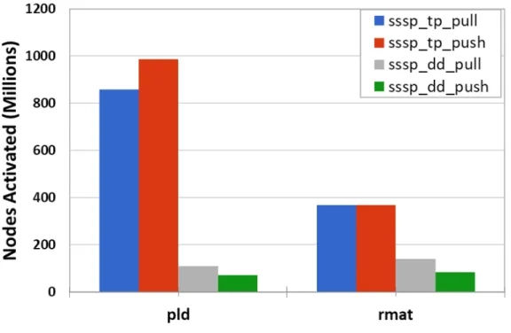
5.26 Total nodes activated for SSSP with pld and rmat graphs. . . 47
5.27 Total edges processed for BFS with pld and graphs. . . 48
5.28 Total nodes activated for BFS with pld and rmat graphs. . . 48
5.29 L2 miss rates for PR with wg, lj, pld, and rmat graphs. . . 50
5.30 L3 miss rates for PR with wg, lj, pld, and rmat graphs. . . 50
LIST OF FIGURES xi
5.32 L3 miss rates for SSSP with wg, lj, pld, and rmat graphs. . . 52
5.33 L2 miss rates for BFS with wg, lj, pld, and rmat graphs. . . 53
5.34 L3 miss rates for BFS with wg, lj, pld, and rmat graphs. . . 53
5.35 L1 miss rates for PR with wg, lj, pld, and rmat graphs. . . 55
5.36 TLB miss rates for PR with wg, lj, pld, and rmat graphs. . . 55
5.37 L1 miss rates for SSSP with wg, lj, pld, and rmat graphs. . . 57
5.38 TLB miss rates for SSSP with wg, lj, pld, and rmat graphs. . . 57
5.39 L1 miss rates for BFS with wg, lj, pld, and rmat graphs. . . 58
5.40 TLB miss rates for BFS with wg, lj, pld, and rmat graphs. . . 58
5.41 Instructions per cycle for PR with wg, lj, pld, and rmat graphs. . 60
5.42 Instructions per cycle for SSSP with wg, lj, pld, and rmat graphs. 60 5.43 Instructions per cycle for BFS with wg, lj, pld, and rmat graphs. . 61
List of Tables
2.1 Summary of frameworks used for graph processing. . . 6
5.1 System details for our experiments. . . 25
5.2 Datasets used for evaluation. . . 26
Chapter 1
Introduction
With the advent of big data applications, graph analytics has gained much impor-tance in recent years. Applications of graph analytics could be applied to a wide range of domains such as biology, robotics, machine learning, and artificial intel-ligence [1]. Moreover, a huge amount of data can be represented as graphs such as biological networks, social networks, road networks, item-product networks, and so on. These networks usually have millions of vertices and billions of edges, and each of which has different structures. Many algorithms are designed to work on graph applications which play a vital role in several domains. For instance, Pagerank (PR) is a popular benchmark for graph analytics applications which is used for ordering hyperlinks as well as evaluating sentence similarity [2]. Fur-thermore, algorithms like Breadth First Search (BFS) and Single-Source Shortest Path (SSSP) are chiefly exercised in cognitive systems embodied various elements from different domains such as machine learning, artificial intelligence, and data analytics. Moreover, Stochastic Gradient Descent (SGD) and Alternating Least Squares (ALS) are two well-known examples of matrix factorization in collabora-tive filtering primarily utilized for personalized recommendation [3]. Additionally, applications of belief propagation are widely adopted in several domains such as bioinformatics, natural language processing, and pattern recognition in order to solve inference problem by passing local messages between nodes.
Over the past decade, researchers have discussed various types of graph appli-cations for finding shortest paths, optimizing routes, discovering cliques among communities, making targeted product recommendations, clustering, and so forth. For this purpose, they have designed many graph processing frameworks [4–8]. However, each framework optimizes the algorithms by adopting different design decisions. Typically, these decisions determine (1) how to order active nodes for computation, (2) how data moves throughout execution, and (3) how to activate nodes. For instance, Pregel [4] adopts bulk synchronous parallel ex-ecution, whereas Graphlab favors asynchronous parallel execution. In terms of information flow, Galois [8] prefers moving data in the push direction, that is to say, an active node performs update operations on its outgoing neighbors. On the other hand, in [9, 10], an active node collects data from its incoming neighbors and updates itself. Moreover, several frameworks utilize a worklist structure for storing nodes activated according to a predefined threshold which need to be pro-cessed [8,11,12]. In contrast, other frameworks process each node according to the graph topology without checking its active status [7,10]. As a consequence, due to the aforementioned design choices for a graph algorithm, there is not a complete and yet effective way to implement large-scale parallel graph applications.
Although the computational capabilities of the computers are increased from teraflops to petaflops and beyond, finding an effective implementation of a graph algorithm executed on different types of graphs has many challenges due to the complex patterns of computation in graph analytics applications, large graph sizes, and diversity in graph structures [13]. Not only the properties of the graphs but also the different memory settings have a huge impact on the per-formance of graph applications [14]. According to recent studies, shared memory implementations show better performance than distributed implementations of graph analytics when graphs fit in the main memory of the system [7, 15, 16]. Communication costs caused by distributed memory settings could not be amor-tized effectively with an increase in memory bandwidth. Moreover, input graphs with billions of edges could easily fit in the main memory of todays large shared memory machines. Therefore, it is important to understand how parallel graph applications can be implemented effectively on shared-memory systems.
1.1
Objective of the Thesis
This thesis analyzes various combinations of different in-memory implementa-tion styles of graph applicaimplementa-tions and explores the tradeoffs between performance, scalability, work efficiency, and computation cost of shared-memory systems. We believe that our observations can guide researchers in making effective choices while implementing future graph analytics applications.
Our main contributions can be summarized as follows:
• We implement 8 variants of the PR algorithm, and 4 variants of both SSSP and BFS algorithms with regards to various design decisions such as the order of computations, data access patterns, and work activation.
• We provide performance and scalability analysis for all implementations using both synthetic graphs as well as real social networks.
• We analyze work efficiency of different design choices by taking the total number of edges processed into consideration.
• Finally, a micro-architectural analysis of the algorithms is conducted so as to reveal the bottlenecks of each algorithm that constraint performance of the shared-memory systems.
1.2
Organization of the Thesis
Chapter 2 covers previous work and summarizes existing graph frameworks by considering their characteristics. Chapter 3 reveals main properties of graph applications and examines various design choices for implementing large-scale graph algorithms. Chapter 4 presents different implementations of PR, SSSP, and BFS.
Chapter 5 is divided into 3 sections. Firstly, experimental setup is presented. In this section, we give the summary of datasets used for evaluation, the details of application design, and the system which experiments are executed on. Sec-ondly, performance and scalability analysis for all applications are given. Their speedups with respect to the running time of a baseline sequential algorithm are also reported. As work efficiency is an important metric, we give the work effi-ciency of each application. In the third section, the performance of the system is evaluated by using hardware performance counters.
Chapter 6 discusses our observations and conclusions from the experimental results. Finally, we conclude the thesis with a brief overview of our work, accom-plishments, and future remarks.
Chapter 2
Related Work
Recently, graph analytics applications have received considerable attention from both industry and academic environments. Many frameworks eliminate major difficulties of graph processing through various abstractions. In this chapter, a short review of those frameworks will be given to illustrate their main differences according to various design choices such as the order of computations, data access patterns, and work activation.
An important design consideration is the target platform while choosing an appropriate framework. While some frameworks target distributed architectures, others focus on shared memory systems. Furthermore, some frameworks allow users to make decisions about data flow (pull or push) and execution order (syn-chronous or asyn(syn-chronous). However, other systems might impose a limit to utilize only a single model. For instance, Pregel [4] uses push-based implemen-tation, while GraphLab [5] uses pull-based. Additionally, some frameworks such as Galois [8] and GraphChi [17] are restricted to asynchronous execution, while GraphLab [5] lets the user decide during implementation. Apart from the design selections regarding information flow and execution order, most frameworks offer a vertex-centric model for programming, although some others such as Ligra [7] uses graph-centric model. Table 2.1 lists different frameworks with their proper-ties including execution model, flow model, and programming model.
There is no clear consensus among the graph processing frameworks on opti-mum design selections, thus benchmarks used for these systems depend on the input data and design decisions that developer enforces. Proper benchmark se-lection is critical in comparing frameworks based on performance criteria such as runtime or scalability. There are graph processing benchmark suites such as GAP [10] and CRONO [18] to encourage the standardization of graph processing evaluations. Table 2.1 summarizes aforementioned graph frameworks with their characteristics.
Table 2.1: Summary of frameworks used for graph processing.
Framework Year System Execution Model
Flow Model
Programming Model Pregel [4] 2010 Distributed Synchronous Push Vertex-Centric GraphLab [5] 2010-12 Both Both Both Vertex-Centric GraphChi [17] 2012 Shared Asynchronous Pull Vertex-Centric Giraph [19] 2012 Distributed Asynchronous Push Vertex-Centric Galois [8] 2013 Shared Synchronous Both Vertex-Centric Ligra [7] 2013 Shared Asynchronous Push Graph-Centric GPS [20] 2013 Distributed Synchronous Push Vertex-Centric
We focus on in-memory implementations of graph algorithms. However, there exist many graph frameworks executed on Flash/SSD platforms such as GraphCHi [17], TurboGraph [21], X-Stream [22], FlashGraph [23], and Grid-Graph [24]. Moreover, some graph frameworks like Medusa [25], Gunrock [26], and CuSha [27] are designed to work on GPU systems. There are also some at-tempts to design specific accelerators for graph processing such as Ozdal et al. [28], GraphOps [29], and Tesseract [30].
Chapter 3
Principal Design Decisions for
Graph Applications
In this chapter, we discuss main characteristics of graph analytics applications and examine several alternatives of design choices for implementing graph algorithms.
3.1
Properties of Graph Applications
Graph analytics applications have received considerable attention recently due to its applicability to different domains such as web graphs, social networks, and protein networks. Designing a large scale efficient graph processing system is a challenging task due to the large volume and the irregularity of communication between computations at each vertex or edge. As a result, several graph analytics frameworks [4, 5, 8, 19, 31, 32] adopting different programming models have been developed.
Graph frameworks process graphs either synchronously or asynchronously. The former is easy to program since it processes data simultaneously and iteratively; whereas, the latter needs to order data updates carefully using latest available
dependent state. Moreover, many graph applications are executed until a conver-gence criterion is satisfied. This behavior is implemented simply by executing all vertices iteratively until the convergence is reached. However, there is no need to execute all vertices in every iteration because some vertices may converge faster than others, causing asymmetric convergence.
We focus on graph algorithms that display three main characteristics:
• We consider vertex-centric algorithms rather than edge-centric or graph-centric. In such applications, a vertex performs local computation on its neighbor vertices (e.g., incoming vertices or outgoing vertices). However, during computation, overlapping neighborhoods might become a bottleneck since they typically need synchronization between threads.
• For each vertex an iterator iterates through its incoming and/or outgoing edges.
• They are iterative and perform a local computation at a set of vertices repeatedly until a convergence criterion is met.
Furthermore, vertex-centric executions can be specialized for different applica-tions. For this purpose, we classify design choices in three orthogonal dimensions as shown in Figure 3.1.
Synchronous Asynchronous
Pull Push Pull-Push
Topology Data-Driven Execution Mode Data Access Pattern Work Activation
Figure 3.1: Algorithm design choices in graph applications.
When applications are designed in a data-driven manner, two additional design choices need to be considered, namely, the structure of a frontier which tracks active nodes and scheduling of frontiers. However, we do not consider these data-driven choices, rather we focus on the first three dimensions. In the following three sections, we describe the aforementioned dimensions in detail.
3.2
Order of Computations
The first dimension is to decide whether to use fine-grain or coarse-grain syn-chronization. One option is synchronous execution that provides synchronization between its iterations by placing barriers. This method eliminates fine grain syn-chronization such as using locks for every vertex or applying atomic operations. The second method employs fine grain synchronization in order to implement ap-plications asynchronously. An algorithm executed asynchronously needs to per-form update operations on the vertices and edges atomically so that sequential consistency will be protected.
In order to avoid any conflict while updating the value of each vertex in parallel, we can use an atomic exchange function as shown in Algorithm 3.1. The function takes three parameters such as an array pointer, an index value, and the desired value. The array pointer and the index value are used for pointing the atomic object which is expected to be updated with the desired value. If the value pointed by the atomic object (e.g., expected[index]) and the non-atomic expected value (e.g., oldVal) are equal, the function atomically exchanges the value of the atomic object with the desired value. Otherwise, the function atomically loads the old value of the atomic object. Therefore, we need an additional statement for ensuring correct exchange operation.
Algorithm 3.1 Atomic Exchange
1: function atomicExchange(∗expected, index, desired) 2: oldVal = expected[index]
3: while !expected[index].compare exchange weak(oldVal,newVal) do
4: oldVal = expected[index]
5: end while
6: end function
Moreover, built-in functions like compare-and-swap (CAS), atomic-min, fetch-and-add can be used for accessing memory atomically. We used atomic exchange and CAS functions in our implementations.
3.3
Data Access Patterns
The second dimension is to select an appropriate data access pattern in which we have three different choices. The first one is a pull-based implementation which indicates the direction of the data movement. An algorithm implemented in the pull direction iterates over incoming (or outgoing) edges to gather their data and executes a reduction with neighbors' data. Note that, this is only a read opera-tion. On the contrary, in push-based implementations, neighbors are updated by the vertex being processed. These write operations are implemented with atomic operations such as compare-and-swap (CAS) primitive. And finally, the pull-push operation has both of the characteristics of pull and push. This implementation iterates over neighbors and reduces their data with atomic operations.
3.4
Work Activation
The third dimension is to select whether to process all vertices at every iteration or only process those vertices with updates. In terms of work activation, imple-mentations are classified into two main types: topology-driven or data-driven.
Topology driven implementation pretends that all graph vertices are active, thus processing each node in every iteration without considering whether some nodes have updates or not. As expected, this causes more computation and in-creased irregular memory accesses, thereby causing inefficiencies. This is more critical especially for graphs which embodies large sparsity. Despite this draw-back, topology driven implementations eradicate the worklist usage for activation. On the other hand, the data-driven model keeps a list of active vertices which are recently updated. Therefore, the algorithm visits the nodes and does the computation according to whether they are on the list or not. This optimization typically prevents unnecessary computations and memory accesses. Data-driven approach is preferable for multicore programming in order to ameliorate the work efficiency. However, the management of work list structure is challenging.
Chapter 4
Implementations of Selected
Graph Algorithms
We implemented 8 different versions of PR algorithm by considering 3 design choices as explained: the order of computations, data access pattern, and work activation. Synchronous techniques used in graph traversal are generally expected to cause performance loss due to load imbalance between bariers [33] when com-pared to their asychronous counterparts. Also, pull-push based methods are not suitable for SSSP and BFS algorithms. For these reasons, we implement 4 dif-ferent versions of SSSP and BFS by considering difdif-ferent combinations of data access patterns and work activations. These applications are designed to be exe-cuted asynchronously due to performance bahaviors. In this chapter, we describe the details of these applications with different parameters.
4.1
Pagerank (PR)
PR is a widely adopted benchmark in many frameworks [7,8,10,15,16,34] since it displays the properties of graph applications as mentioned in the previous chapter. In addition, it captures the irregular memory access, work scheduling, and load
imbalance characteristics of many graph algorithms. Algorithm 4.1 gives the details of base PR algorithm.
Algorithm 4.1 Topology-driven Pull-based Synchronous PR Input: G = (V,E)
Output: scores
1: scores[:] = 1.0 − α
2: for i until maxIter do
3: activeNum = 0 4: parfor v ∈ V do 5: sum = 0 6: for w ∈ inNeighbor(v) do 7: sum += scores[w]/outDegree(w) 8: end for 9: nextScores[v]=(1.0 − α) + α*sum
10: if fabs(nextScores[v] - scores[v]) ≥ ε) then
11: activeNum++ 12: end if 13: end parfor 14: swap(scores, nextScores) 15: if activeNum ≤ 0 then 16: break 17: end if 18: end for 19: scores = scores / | V |
In terms of execution, PR can be performed both synchronously and asyn-chronously. As shown in Equation 4.1, power method [2] can be employed in order to calculate rank values in a synchronous manner. This method holds both current and previous ranks of each vertex. In each iteration, a vertex calculates its new rank by using ranks which are calculated in the previous iteration.
P rt+1[u] = α × X
w∈w→u
P rt[w]
Tw
+ (1 − α) (4.1)
On the other hand, PR algorithm can be performed asynchronously by employ-ing Gauss-Seidel method [35] as shown in Equation 4.2 In this case, each vertex updates its rank by utilizing the most recent ranks calculated. For each vertex,
only the most up-to-date rank is stored and iterations are not separated by bar-riers; therefore, iterations are not clearly defined in asynchronous applications. In parallel implementations, PR algorithm implemented by using Gauss-Seidel formulation should synchronize threads because one thread might try to write a recently calculated rank for a vertex while a different thread might try to read the rank of the same vertex.
P rt+1[u] = α × X w∈w→u P rt[w] Tw + X v∈v→u P rt+1[v] Tv ! + (1 − α) (4.2)
In terms of data access patterns, PR applications can be implemented in three different ways, namely pull, push, and pull-push. Pull-based PR can be imple-mented both synchronously and asynchronously; however, push-based and pull-push based versions should be implemented by Gauss-Seidel [35]. Synchronous pull-based applications utilize two lists for keeping current and next ranks of each vertex, and in each iteration, a vertex can only see the ranks of its in-neighbors from previous iterations. Moreover, each vertex pulls the ranks of its incoming neighbors and updates itself only once per step. Therefore, pull-based applica-tions do not require synchronization since the elements of the list are updated only once in an iteration. In contrast, asynchronous pull-based applications use only one list in order to keep ranks of each vertex. For this reason, they need an exclusive lock for writing and updating data since more than one write is issued for some vertices at the same time.
From work activation perspective, PR applications can be implemented in both styles such as topology-driven and data-driven. We combined these two work ac-tivation schemes with all data-access patterns as mentioned before. Algorithms 4.3 and 4.4 illustrate how an active node accesses its neighbours in the push di-rection and pull-push didi-rection, respectively. As can be seen in Algorithm 4.4, after an active node accesses its in-neighbors to gather their contributions, the active node updates its out-neighbors’ rank immediately. Therefore, total work done in pull-push based method, is augmented. Furthermore, using a worklist, we
track each active vertex by utilizing bit vector structures in data-driven applica-tions. As an alternative, we also implemented a worklist based on a central queue structure by using lock primitives. However, in our experiments, both worklist structures exhibit similar performance. For this reason, we only report the results for bit vector implementation.
Algorithm 4.2 Data-Driven Pull-based Asynchronous PR Input: G = (V,E) Output: ranks 1: aRanks[:] = 1.0 − α 2: frontier[:] = true 3: next[:] = false
4: for i until maxIter do
5: activeNum = 0 6: parfor v ∈ V do 7: if frontier[v] then 8: sum = 0 9: for w ∈ inNeighbor(v) do 10: sum += aRanks[w]/outDegree(w) 11: end for 12: oldRank = aRanks[v] 13: newRank =(1.0 − α) + α*sum 14: atomicExchange(aRanks, v, newRank)
15: if fabs(newRank - oldRank) ≥ ε) then
16: for w ∈ outNeighbor(v) do 17: if !next[w] then 18: next[w] = true 19: end if 20: end for 21: activeNum++ 22: end if 23: end if 24: end parfor 25: swap(frontier, next) 26: next[:] = false 27: if activeNum ≤ 0 then 28: break 29: end if 30: end for 31: ranks = aRanks / | V |
Algorithm 4.3 Data-Driven Push-based Asynchronous PR Input: G = (V,E) Output: ranks 1: parfor v ∈ V do 2: ranks[v] = 1.0 − α 3: aResiduals[v] = 0.0 4: frontier[v] = true 5: next[v] = false 6: for w ∈ inNeighbor(v) do 7: aResiduals[v] + = 1.0/ outDegree(w) 8: end for 9: aResiduals[v] = (1.0 − α) ∗ α∗aResiduals[v] 10: end parfor
11: for i until maxIter do
12: activeNum = 0 13: parfor v ∈ V do 14: if frontier[v] then 15: ranks[v] += aResiduals[v] 16: delta = α∗(aResiduals[v]/outDegree(v)) 17: for w ∈ outNeighbor(v) do 18: oldRes = aResiduals[w]
19: atomicExchange(aResiduals, w, oldRes + delta)
20: if fabs(oldRes + delta ≥ ε&& oldRes ≤ ε) then
21: activeNum++ 22: if !next[w] then 23: next[w] = true 24: end if 25: end if 26: end for 27: aResiduals[v] = 0.0 28: end if 29: end parfor 30: swap(frontier, next) 31: next[:] = false 32: if activeNum ≤ 0 then 33: break 34: end if 35: end for 36: ranks = ranks / | V |
Algorithm 4.4 Data-Driven Pull-Push-based Asynchronous PR Input: G = (V,E) Output: ranks 1: parfor v ∈ V do 2: aRanks[v] = 1.0 − α 3: aResiduals[v] = 0.0
4: frontier[v] = true, next[v] = false
5: for w ∈ inNeighbor(v) do
6: aResiduals[v] + = 1.0/ outDegree(w)
7: end for
8: aResiduals[v] = (1.0 − α) ∗ α∗aResiduals[v]
9: end parfor
10: for i until maxIter do
11: activeNum = 0 12: parfor v ∈ V do 13: if frontier[v] then 14: sum = 0 15: for w ∈ inNeighbor(v) do 16: sum += aRanks[w]/outDegree(w) 17: end for 18: newRank = (1.0 − α + α∗)sum 19: atomicExchange(aRanks, v, newRank) 20: delta = α∗(aResiduals[v]/outDegree(v)) 21: for w ∈ outNeighbor(v) do 22: oldRes = aResiduals[w]
23: atomicExchange(aResiduals, w, oldRes + delta)
24: if fabs(oldRes + delta ≥ ε&& oldRes ≤ ε) then
25: activeNum++ 26: if !next[w] then 27: next[w] = true 28: end if 29: end if 30: end for 31: aResiduals[v] = 0.0 32: end if 33: end parfor 34: swap(frontier, next) 35: next[:] = false 36: if activeNum ≤ 0 then 37: break 38: end if 39: end for 40: ranks = aRanks / | V |
4.2
Single-Source Shortest Path (SSSP )
In the single source shortest path (SSSP) problem, we try to find minimum cost path from a single source node to all other nodes in a weighted directed graph. A well-known sequential algorithm to solve the SSSP problem is Dijkstra's algo-rithm [36]. A parallel algoalgo-rithm, called delta-stepping [37, 38], divides Dijkstra's algorithm into buckets which can be executed in parallel. The alternative parallel algorithm for solving the SSSP problem is Bellman-Ford [39] which allows nega-tive edge weights. Our SSSP implementations are adopted from this algorithm.
We implemented four different versions of SSSP algorithm by considering dif-ferent data access patterns and work activation choices. Note that, SSSP is im-plemented asychronously since their synchronous implementations are expected to show poor perforamance as explained in literature [33, 38]. As shown in Al-gorithm 4.5, in pull-based applications, an active node updates its distance by pulling (reading) data from its incoming neighbors. The write operation is only performed on the active node. However, in push-based applications, data flows from the active node to its outgoing neighbors. Since the active node updates its outgoing neighbors distances by pushing its distance value to its outgoing neighbors, push-based applications generate more frequent updates.
We provide the pseudo code for both pull-based and push-based versions as shown in Algorihtms 4.5 and 4.6, respectively. Both of them employ bit vectors in order to keep track of active vertices for each iteration. Each algorithm iterates until there is no change in the distance value of any node. As explained before, vertex updates are performed asynchronously.
Algorithm 4.5 Data-Driven Pull-based SSSP Input: G = (V,E), source, w
Output: dists
1: aDists[:] = +∞
2: frontier[:], next[:] = false
3: dists[source] = 0
4: frontier[source] = true
5: for v ∈ outNeighbor(source) do
6: frontier[v] = true
7: end for
8: for i until maxIter do
9: activeNum = 0
10: parfor u ∈ V do
11: minDist = +∞
12: for v ∈ inNeighbor(u) do
13: if minDist > aDists[v] + w(v,u) then
14: minDist = aDists[v] + w(v,u)
15: end if
16: end for
17: if aDist[u] > minDist then
18: atomicExchange(aDist, u, minDist) 19: for v ∈ outNeighbor(u) do 20: if !next[v] then 21: next[v] = true 22: end if 23: end for 24: activeNum++ 25: end if 26: end parfor 27: swap(frontier, next) 28: next[:] = false 29: if activeNum ≤ 0 then 30: break 31: end if 32: if activeNum ≤ 0 then 33: break 34: end if 35: end for 36: dist = aDists
Algorithm 4.6 Data-Driven Push-based SSSP Input: G = (V,E), source, w
Output: dists
1: aDists[:] = +∞
2: frontier[:], next[:] = false
3: aDists[source] = 0
4: frontier[source] = true
5: for i until maxIter do
6: activeNum = 0
7: parfor u ∈ V do
8: if frontier[u] then
9: for v ∈ outNeighbor(u) do
10: if aDists[v] > aDists[u] + w(u,v) then
11: newDist = aDists[u] + w(u,v)
12: atomicExchange(aDists, v, newDist ) 13: activeNum++ 14: if !next[v] then 15: next[v] = true 16: end if 17: end if 18: end for 19: end if 20: end parfor 21: swap(frontier, next) 22: next[:] = false 23: if activeNum ≤ 0 then 24: break 25: end if 26: end for 27: dist = aDists
4.3
Breadth-First Search(BFS )
As a well-known algorithm, in breadth-first search (BFS), the goal is to find the breadth-first order traversal of the graph vertices. BFS is similar to SSSP in which edge weights are set to be 1 instead of using weights from the input. Similar to SSSP, our BFS implementations also follow the logic in Bellman-Ford [39].
We have implemented four different versions of BFS by considering two differ-ent design choices, namely, data access pattern and work activation. As shown in Algorithm 4.7, pull-based version executes a reduction over incoming edges and finds the minimum level of neighbors, then corresponding vertex level is up-dated accordingly. On the other hand, Algorithm 4.8 illustrates a push-based implementation where outgoing neighbors update their level by using atomic op-erations. Different BFS implementations follow the same pattern as in SSSP, except the fact that edge weight is always 1. Moreover, BFS applications are de-signed to be executed asynchronously since recent studies show that asynchronous implementations show better performance than their synchronous counterparts [40].
Algorithm 4.7 Data-Driven Pull-based BFS Input: G = (V,E), source
Output: levels
1: aLevels[:] = +∞
2: frontier[:], next[:] = false
3: dists[source] = 0
4: frontier[source] = true
5: for v ∈ outNeighbor(source) do
6: frontier[v] = true
7: end for
8: for i until maxIter do
9: activeNum = 0
10: parfor u ∈ V do
11: minLevel = +∞
12: for v ∈ inNeighbor(u) do
13: if minLevel > aLevels[v] + 1 then
14: minLevel = aLevels[v] + 1
15: end if
16: end for
17: if aLevels[u] > minLevel then
18: atomicExchange(aLevels, u, minLevel) 19: for v ∈ outNeighbor(u) do 20: if !next[v] then 21: next[v] = true 22: end if 23: end for 24: activeNum++ 25: end if 26: end parfor 27: swap(frontier, next) 28: next[:] = false 29: if activeNum ≤ 0 then 30: break 31: end if 32: if activeNum ≤ 0 then 33: break 34: end if 35: end for 36: levels = aLevels
Algorithm 4.8 Data-Driven Push-based BFS Input: G = (V,E), source
Output: aLevels
1: aLevels[:] = +∞
2: frontier[:], next[:] = false
3: aLevels[source] = 0
4: frontier[source] = true
5: for i until maxIter do
6: activeNum = 0
7: parfor u ∈ V do
8: if frontier[u] then
9: for v ∈ outNeighbor(u) do
10: if aLevels[v] > aLevels[u] + 1 then
11: newLevel = aLevels[u] + 1 12: atomicExchange(aLevels, v, newLevel) 13: activeNum++ 14: if !next[v] then 15: next[v] = true 16: end if 17: end if 18: end for 19: end if 20: end parfor 21: swap(frontier, next) 22: next[:] = false 23: if activeNum ≤ 0 then 24: break 25: end if 26: end for 27: levels = aLevels
Chapter 5
Experiments
5.1
Experimental Setup
We conducted our experiments on a multi-socket server system with specifications given in Table 5.1. All algorithms are implemented using C++ and OpenMP, and the datasets are stored in Compressed Sparse Row (CSR) format [41]. For each vertex, we store their in-neighbors and out-neighbors in separate sets in order to improve locality. The runtime is the average results of 10 runs, and it includes the time for allocation and initialization of all data structures for each algorithm (except initial graph itself). We use Performance API (PAPI) [42] in order to access hardware counters in the system, thereby observing the characteristics of underlying architecture.
Table 5.1: System details for our experiments.
Component Specification
CPU Intel Xeon E5-2643 @3.30GHz, 8 cores,
2 sockets, 4 cores/socket, 2 threads/core
Cache Private 32 KB L1 cache, Private 256KB L2 caches
Shared 10MB L3 cache
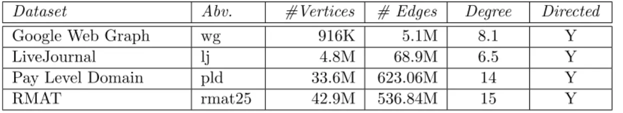
We evaluate the implementations of all design alternatives using the datasets in Table 5.2. Our testbed involves both small graphs as well as large graphs. For our synthetic data sets, RMAT graph is generated with parameters (A,B,C) = (0.45, 0.25, 0.15) by using Graph500 benchmarks [43]. Pay Level Domain is a hyperlink graph obtained from the Common Crawl web corpora [44]. We select Google Web Graph (wg), and soc-LiveJournal (lj) from the SNAP datasets [45]. All graphs are directed and duplicate edges are removed.
Table 5.2: Datasets used for evaluation.
Dataset Abv. #Vertices # Edges Degree Directed Google Web Graph wg 916K 5.1M 8.1 Y
LiveJournal lj 4.8M 68.9M 6.5 Y
Pay Level Domain pld 33.6M 623.06M 14 Y
RMAT rmat25 42.9M 536.84M 15 Y
In this work, we implement 16 different versions of 3 algorithms by consider-ing different design decisions. The detailed summary of design choices for each application is found in Table 5.3.
Table 5.3: Summary of application test cases.
Algorithm Application # Activation # Access Execution pr tp pull syn topology pull synchronous pr, sssp, bfs tp pull asyn topology pull asynchronous pr, sssp, bfs tp push topology push asynchronous pr td pull push topology pull-push asynchronous pr dd pull syn data-driven pull synchronous pr, sssp, bfs dd pull asyn data-driven pull asynchronous pr, sssp, bfs dd push data-driven push asynchronous pr dd pull push data-driven pull-push asynchronous
5.2
Performance Results
This section presents performance analysis of the implementations in terms of execution time and scalability. Moreover, we report speedups of the algorithms relative to the best serial execution in each dataset.
5.2.1
Runtime and Scalability
5.2.1.1 PR
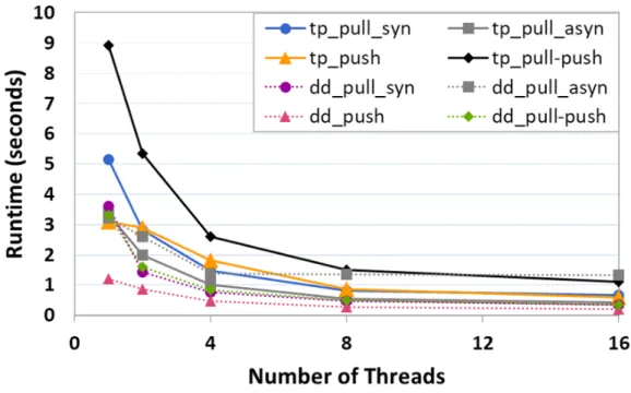
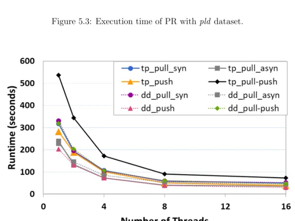
Figures 5.1-4 show the performance of different implementations of PR in terms of execution time with respect to the number of threads. These figures illustrate that among all implementations, topology driven pull-push-based methods have poor performance when compared to both pull-based and push-based methods. This is expected as pull-push-based methods require reading operations on in-neighbors as well as write operations on out-neighbors. However, in pull-based methods, a vertex performs only one update operation on itself and performs many read operations on its incoming edges. Likewise, push-based methods perform only write operations on itself and its out-neighbors instead of requiring both read and write operations on its neighbors as in pull-push-based methods.
Since pull based methods require only one write and many read operations, they are expected to be more cache friendly. Nevertheless, as shown in Figures 5.1-4, topology driven pull-based methods give the second-worst performance among all implementation styles. Although push-based methods require more frequent write operations, data-driven push-based methods are the fastest among all implementation variants for all datasets. One reason for such behavior is that push-based methods accelerate the rate of the dissemination of information, hence they can amortize the overhead required for frequent writes. However, this is not the case for topology driven push-based methods. Figures 5.1 and 5.2 show that quick frequent updates on ranks do not improve the performance of topology driven push-based methods sufficiently because they need to iterate
over all the nodes without checking their activation status. As a matter of fact, these frequent updates increase the number of nodes activated in topology based implementations of other algorithms such as SSSP and BFS.
Our observations also show that the performance of data-driven methods is better than the performance of topology driven ones. This result is also consistent with the observations in [46]. Data-driven methods employ a worklist in order to keep active nodes whose ranks change more from a defined threshold, hence they can filter out many edges instead of processing them unnecessarily. As can be seen in Figures 5.1-4, the effectiveness of employing a frontier for tracking active nodes can be clearly seen by looking at the performance improvement of the pull-push based method. When utilizing an active list, the run time of the algorithms decreases drastically compared to topology driven ones as illustrated in Figure 5.3.
Next, we consider the choice of executing the applications with asynchronous execution model. The results demonstrate that if we execute a method asyn-chronously, its performance improves. Although asynchronous executions require atomic operations, they are able to mitigate synchronization overheads by accel-erating convergence rate of the algorithm. For instance, pull-based asynchronous applications perform better compared to their synchronous counterparts on large graphs as shown in Figures 5.3 and 5.4. However, on small graphs, Figures 5.1 and 5.2 show that only their topology-driven pull-based versions outperform their synchronous versions. When applications use a worklist for tracking active nodes, synchronous versions deliver higher performance than their asynchronous coun-terparts on small graphs. One possible drawback of synchronous execution is due to the slow convergence rate. In each iteration, a vertex can only see the update from previous iteration, hence the information is disseminated more slowly when compared to the methods executed in Gauss-Seidel way. In asynchronous models, the order of updates is not separated with barriers and only one global list is used for keeping rank values. As a result, each vertex can detect the most up-to-date version of data which increases the convergence rate of the algorithms.
Figure 5.1: Execution time of PR with wg dataset.
Figure 5.3: Execution time of PR with pld dataset.
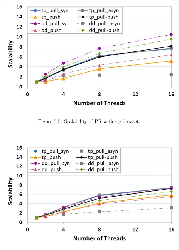
Scalability is used as another performance metric which measures a parallel system’s capacity to increase speedup with respect to the number of threads. For this purpose, the scalability of different implementations of PR is given in Figures 5.5-8. In these figures, Y-axis indicates self-relative scalability, and X-axis represents the number of threads. For all datasets, asynchronous data-driven pull-based methods perform the poorest scalability although other alternatives of pull-based methods scale very well. Both synchronous and asynchronous variants of topology driven pull-based methods exhibit good scalability. However, for data-driven pull-based methods, asynchronous versions have much less scalability than the synchronous ones as shown in Figures 5.5-8. This indicates that mode of execution becomes significant when the algorithm is implemented in a data-driven way.
As can be seen in Figures 5.7 and 5.8, for large graphs, all classes of algorithms except the asynchronous data-driven pull-based ones are highly scalable. Interest-ingly, although the topology-driven pull-push-based methods display the poorest performance, they show the best scalability. Moreover, data-driven push-based methods show slightly less scalability for pld graph. For small graphs, we observe a different pattern in scalability when compared to the large graphs. Push-based methods show the second-poorest scalability. One possible reason is the fact that push-based methods require frequent write operations on out-neighbors, thereby limiting the scalability. On the other hand, the scalability of pull-push based methods are significantly high, especially for large graphs as shown in Figures 5.7 and 5.8.
Figure 5.5: Scalability of PR with wg dataset.
Figure 5.7: Scalability of PR with pld dataset.
5.2.1.2 SSSP
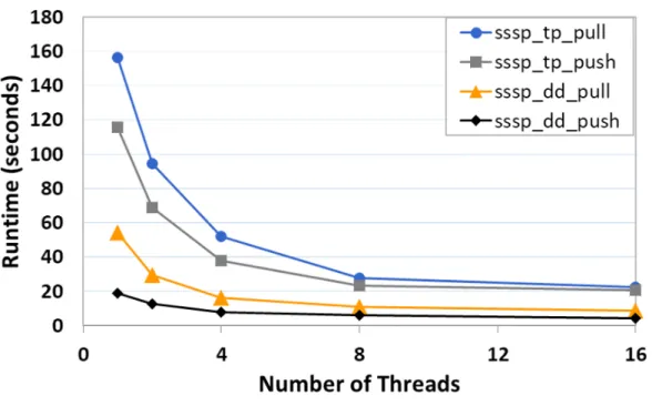
Figures 5.9-10 and 5.11-12 indicate execution time and scalability of different imlementations of SSSP algorithm. Among all variants of SSSP, topology-driven based methods show less performance than data-driven methods as shown in Fig-ures 5.9 and 5.10. By contrast, the implementations which employ topology-based activation scheme are highly scalable. We observe that data-driven implementa-tions are also scalable but their scalability is low compared to the topology-driven alternatives. Although data-driven push-based methods are faster than topology-driven pull based methods, both methods perform similar scalability.
For different data access patterns, work activation plays a significant role in the performance and scalability of the algorithms. For push-methods, activation scheme has a huge impact on both performance and scalability. If nodes are activated according to the structure of a graph, then the algorithm shows less performance but high scalability. In contrast, if nodes are activated by utilizing a frontier, the algorithm has better performance but it shows relatively low scal-ability. This observation is valid for all datasets except rmat graph as shown in Figure 5.12. All variants of SSSP algorithm demonstrates similar scalability with respect to one another on rmat graph.
Figure 5.9: Execution time of SSSP with pld dataset.
Figure 5.11: Scalability of SSSP with pld dataset.
5.2.1.3 BFS
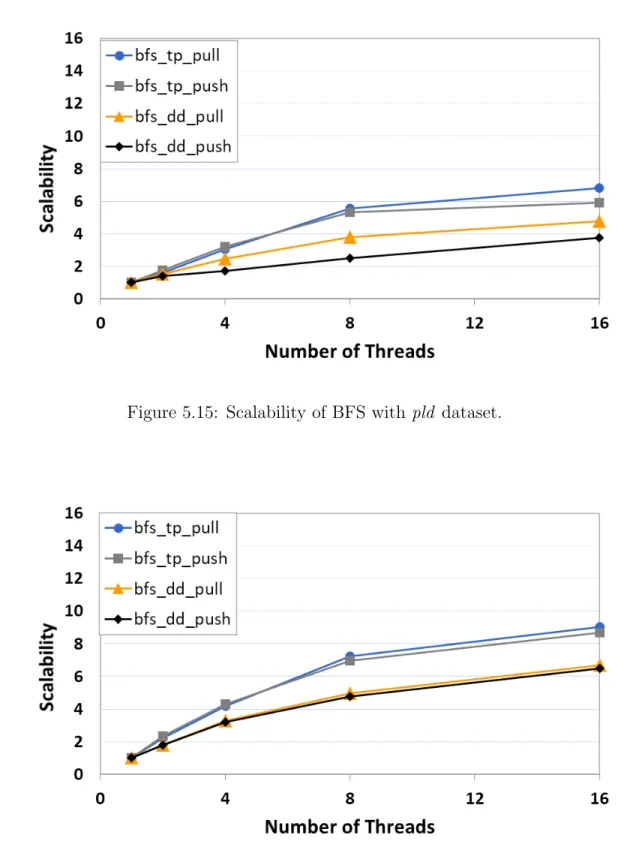
BFS implementations exhibit similar performance when compared to SSSP. For both classes, data-driven methods are faster than topology-driven methods, and push-based alternatives outperform pull-based alternatives as illustrated in Fig-ures 5.13 and 5.14. Moreover, FigFig-ures 5.15 and 5.16 show that scalability of data-driven methods is lower than the scalability of topology-driven ones. The increase in the number of threads improves the performance of all algorithms. One interesting observation which can be seen from Figure 5.16 is that the effect of data access patterns such as pull vs. push on scalability of the algorithms on rmat graph is negligible.
Figure 5.13: Execution time of BFS with pld dataset.
Figure 5.15: Scalability of BFS with pld dataset.
5.2.2
Speedups
In this section, we report speedups for the aforementioned implementations of PR, SSSP, and BFS. For brevity, we only report speedups on large graphs which are still valid for small graphs. We normalize the execution time speedups to the synchronous topology-driven pull-based method since it is a widely used bench-mark in previous studies. For PR, the base case corresponds to the power method as shown in Equation 4.1.
As already mentioned in the previous chapter, data-driven push-based meth-ods provide the highest performance in all the experiments. For PR algorithm, Figures 5.17 and 5.18 demonstrate that speedups of work efficient push based implementations are 35x and 11x for pld and rmat graphs, respectively. The least speedups are gained from topology-driven pull-push-based methods. Never-theless, if pull-push based methods are implemented in a data-driven way, they deliver substantial speedups over their topology-driven versions. For instance, on pld graph, the speedup of pull-push-based implementation increases from 5x to 18x when a worklist is used in order to track previously visited nodes.
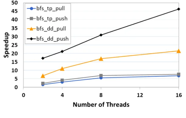
As can be seen in Figures 5.19-20 and 5.21-22, all implementations of SSSP and BFS algorithms show at least 7x speedup relative to the baseline implemen-tation in 16 threads. For SSSP and BFS applications, significantly high speedups are obtained in pld and rmat graphs when the algorithms utilize a worklist and do computations in the push direction. Figures 5.19 and 5.21 illustrate that for pld graph, speedups of SSSP and BFS algorithms in 16 threads are 38x and 46x, respectively. Similarly, as shown in Figures 5.20 and 5.22, for rmat graph, speedups of SSSP and BFS algorithms in 16 threads are 19x and 40x, respec-tively. Although BFS algorithm is implemented in a data-driven push-based way, it delivers substantial speedups for both datasets when compared to other im-plementations. On the other hand, all classes of data-driven implementations of SSSP algorithm delivers higher speedups than all topology-based versions. We also notice that data access patterns do not have a huge impact on speedups of SSSP and BFS when the algorithm activates each node in every iteration.
Figure 5.17: Speedups observed for PR with pld dataset.
Figure 5.19: Speedups observed for SSSP with pld dataset.
Figure 5.21: Speedups observed for BFS with pld dataset.
5.2.3
Work Efficiency
In Section 5.2.1, we observed that the performance of data-driven methods is bet-ter than the performance of topology driven ones. Also, the authors showed when asymmetric convergence is enabled in PR algorithm, the total number of edges processed is reduced by 47 percent on average [47]. Therefore, work efficiency can be an important metric for analyzing the performance of graph applications. For these reasons, we provide two different metrics in order to calculate work ef-ficieny. First, we keep a track of edges processed since it captures the number of memory accesses and multiply-add operations applied on edges. The second met-ric is the number of nodes activated during the execution of an application. For topology-driven applications, since the number of edges processed per step and nodes activated per step are constant, total work done is calculated by multiplying the number of edges/nodes of an input graph with the number of iterations.
Our first observation is that data-driven push-based application is the most work efficient implementation among all applications as shown in Figures 5.23 and 5.24. Similarly, we already seen that data-driven push-based application is the fastest one as shown in Figures 5.3 and 5.4. These two findings are consistent with each other since data-driven push-based application performs the least work, hence it shows the best performance.
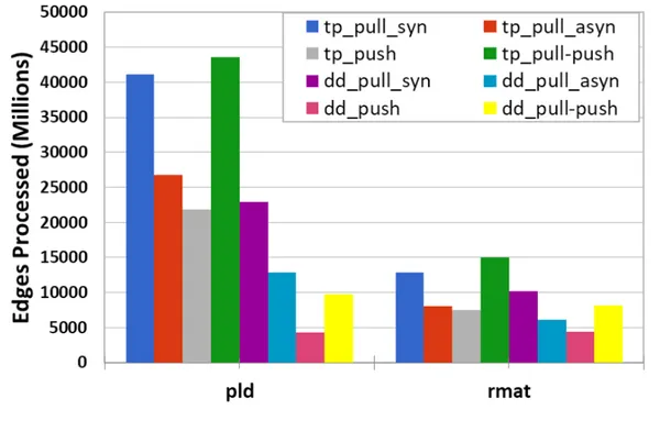
As shown in Figures 5.23 and 5.24, when applications use a worklist in order to track active vertices, they reduce the number of edges processed significantly. Especially, data-driven applications of both SSSP and BFS reduce their total work done in a substantial amount relative to topology-driven pull-based appli-cations. Similarly, as shown in Figures 5.25 and 5.27, data-driven applications implemented in the push and pull-push direction process 5.1x and 4.5x fewer edges on pld graph. As a result, they perform better than their topology-driven versions. This observation is important since when applications become work efficient, they can utilize cache better, thereby improving performance.
Figure 5.23: Total edges processed for PR with pld and rmat graphs.
Data access patterns affect the number of edges processed when applications do not consider activation status of a node. As can be seen in Figure 5.24, both push-based and pull-push based methods activate the same number of nodes; however, Figure 5.23 shows that the pull-push based method processes more edges than the push-based method. Although pull-push based application speeds up the convergence rate of the algorithm like push-based method, it does extra work on incoming edges as shown in Figure 5.24. Since the number of edges processed changes the number of memory accesses, the increase in work done results in poor performance. Similarly, pull-push based methods process more edges in spite of activating less nodes than pull-based method as illustrated in Figures 5.23 and 5.24, respectively. Likewise, Figures 5.25 and 5.27 show that push-based applications of SSSP and BFS process less number of edges when compared to their pull-based counterparts. Additionaly, topology driven push-based versions of SSSP and BFS algorithms are very inefficient in terms of total nodes activated.
Figure 5.25: Total edges processed for SSSP with pld and rmat graphs.
Figure 5.27: Total edges processed for BFS with pld and graphs.
5.3
Microarchitectural Results
In this section, we discuss cache behavior of the aforementioned applications. In addition, we present the rate of translation lookaside buffer (TLB) miss rates and the average number of instructions executed per cycle (IPC) for each applica-tion. We evaluate the performance of the system by using hardware performance counters.
5.3.1
L2/L3 Miss Rates
Although there are many factors to consider when determining performance, it is not clear which application shows better performance. For this purpose, we analyze cache behavior for different implementations explained earlier.
We implement pull, push, and pull-push variants of PR algorithm for each work activation model. Although each application shows different performance, the variations between their L3 miss rates is negligible. We observe that type of an application does not affect the L3 significantly but the graph size for the application being used is directly proportional to the number of L3 misses. For instance, L3 miss rates are less than 55% on small graphs, whereas they are higher than 75% on large graphs, as shown in Figure 5.30.
For all applications, we obtain significantly higher L2 miss rates which are be-yond 80%. In spite of low hit rates, we observe that push-based implementations result in lower L2 hit rates on all graphs, as shown in Figure 5.29. In addition, lj graph delivers lower L2 miss rates for all applications except push-based versions when compared to the other input graphs.
Figure 5.29: L2 miss rates for PR with wg, lj, pld, and rmat graphs.
Figures 5.32 and 5.34 demonstrate that SSSP and BFS applications show a similar pattern with PR application when L3 miss rates are considered. When the size of input graph increases, the total miss rate increases. However, for small graphs, it does not go over 50%. Likewise, all variants of SSSP and BFS generate high miss rates like PR. The highest hit rates for all applications are obtainted with lj graph among all input graphs. However, same observations made for PR are still valid for SSSP and BFS applications as shown in Figures 5.31-32 and Figures 5.33-34, respectively.
Figure 5.31: L2 miss rates for SSSP with wg, lj, pld, and rmat graphs.
Figure 5.33: L2 miss rates for BFS with wg, lj, pld, and rmat graphs.
5.3.2
L1/TLB Miss Rates
For PR algorithm, we notice that pull-based implementations show high L1 miss rates when compared to push and pull-push based variants, as shown in Fig-ure 5.35. Especially, L1 hit rates become worse when a pull-based algorithm is executed synchronously.
Work activation does not make much difference for different application coun-terparts except asynchronous pull-based applications. For instance, L1 miss rates for both synchronous pull, push, and pull-push based applications are slightly dif-ferent from each other. However, L1 hit rates decrease when an asynchronous pull-based algorithm is implemented by utilizing a worklist structure.
We expect pull-based applications to be cache friendly since they perform fre-quent read operations on in-edges and only perform one update operation. How-ever, our findings show the opposite of this expectation. Push-based applications achieve higher hit rates when compared to their pull-based versions. Further-more, all variants of applications show low L1 and TLB miss rates. One reason for the decrease in miss rates when compared to L2/L3 miss rates is the regular accesses thanks to edge lists. For each application, we keep two separate lists for in-edges and out-edges per vertex so applications can benefit from increased spatial locality.
As can be seen from Figure 5.36, patterns observed for L1 miss rates for each data access modes are also valid for TLB miss rates. Moreover, TLB miss rates increase with dataset sizes, as expected, since the bigger the data the higher the number of pages to store. This situation puts more pressure on TLB entries, and as a result, TLB entries are evicted more frequently.
Figure 5.35: L1 miss rates for PR with wg, lj, pld, and rmat graphs.
Similar to PR, SSPP and BFS show similar behavior on L1 and TLB miss rates, as can be seen in Figures 5.37 and 5.38 for SSSP and in Figures 5.39 and 5.40 for BFS. Total L1 and TLB miss rates improve when compared to L2/L3 miss rates. Secondly, push-based applications have higher L1 and TLB hit rates in contrast to pull-based applications. Moreover, similar to PR, TLB miss rates improve on small graphs, whereas they worsen on large graphs.
Finally, L1 and TLB rates have same patterns for each data access pattern. Moreover, we observed that wg and pld graphs are more responsive than lj and rmat graphs to work activation. As shown in Figures 5.38 and 5.40, when an application is designed in a data-driven way, both pull-based and push-based implementations on wg and pld graphs improve their L1 and TLB miss rates.
Figure 5.37: L1 miss rates for SSSP with wg, lj, pld, and rmat graphs.
Figure 5.39: L1 miss rates for BFS with wg, lj, pld, and rmat graphs.
5.3.3
Instructions Per Cycle (IPC)
We also measure the number of instructions that each application execute per clock cycle. For PR applications, we observe a similar pattern on each input graph as shown in Figure 5.41. On the other hand, Figures 5.42 and 5.43 illustrate that SSSP and BFS applications show different behaviors with regards to the graph size. For instance, for all experiments except SSSP and BFS applications applied on small graphs, the overall IPC rates do not exceed 0.2. However, all variants of SSSP and BFS applications have an IPC value of more than 0.2, on small datasets.
Asynchronous data-driven pull-based method obtains the least IPC among all applications of PR as shown in Figure 5.41. By contrast, IPC values decrease for SSSP and BFS methods when they are data-driven as illustrated in Figures 5.42 and 5.43, respectively. Although applications have lower IPC on rmat graph compared to pld, they perform better for all implementations. In other words, maximizing IPC values does not improve performance. More specifically, best IPC value gives the worst results. For instance, for BFS and SSSP, IPC values are inversely proportional to execution times on small graphs as shown in Figures 5.42 and 5.43.
Figure 5.41: Instructions per cycle for PR with wg, lj, pld, and rmat graphs.
Chapter 6
Discussion
We implemented eight different versions of PR algorithm by considering three de-sign choices, namely, the order of computations, data access patterns, and work activation. Moreover, we implemented four different versions of SSSP and BFS by taking different combinations of data access patterns and work activations into account. We analyzed various combinations of different in-memory implementa-tion styles of graph applicaimplementa-tions and explored the tradeoffs between performance, scalability, work efficiency, and computation cost of shared-memory systems.
Initially, we examine the performance and scalability of each application. First observation we made is that, the increase in the number of threads improves the performances of all algorithms as expected. For different data access patterns, work activation appears as a critical indicator which influences the performance and scalability of the algorithms. Moreover, we observed that data-driven push-based methods exhibit the highest performance amongst all the experiments. The least speedups are obtained from topology-driven pull-push-based methods. Nevertheless, work efficient pull-push based methods outperform their topology-driven versions by delivering substantial speedups. In addition, BFS implemen-tations perform similar performance with the corresponding implemenimplemen-tations of SSSP in terms of design decisions. For both classes, data-driven methods lead to a reduction in runtime in comparison with topology-driven methods, while fully
push-based alternatives outperform pull-based alternatives.
Secondly, we also noticed that if the activation of nodes is induced according to the structure of a graph, then the algorithm gives lower performance but high scalability. In contrast, if nodes are activated by utilizing a frontier, the algorithm performs well but it shows relatively low scalability in return. Next, when we in-vestigated the decision of executing the applications with asynchronous execution model, the results demonstrated that if we execute a method in an asynchronous fashion, its performance improves. Although asynchronous executions require atomic operations, they are able to mitigate synchronization overheads by accel-erating convergence rate of the algorithm.
Thirdly, we provided two different metrics in order to calculate work done such as total edges processed and total nodes activated. Our first observation was that data-driven push-based application is the most work efficient implementation among all applications. We noticed that data-driven push-based applications are performing much better due to the fact that they process the least number of edges and activate the least number of nodes. Moreover, data access patterns affect the number of edges processed when applications do not consider activation status of a node.
For determining micro-architectural bottlenecks, we reported cache behaviors of the aforementioned applications. In addition, we presented the rate of trans-lation lookaside buffer (TLB) misses and the average number of instructions executed per cycle (IPC) for each application by using hardware performance counters.
Overall, optimizing graph applications for generally accepted metrics may not give the best performing implementation style. Let us consider scalability as an example. As noted before, pull-based implementations give the best scalability but it does not yield the best performance. On the other hand, data locality characteristics are mostly dependent on the size of datasets rather than details of the implementation. Moreover, for cache levels closer to main memory, the miss rates are quite high.
Furthermore, we observed a relation between data access patterns and work processing order and the performance. For all applications, choosing push based implementation combined with a frontier work activation model gives the best performance. In order to inspect the reason behind this, we have measured the amount of work performed by these implementations for which we have used number of edges processed as a proxy. These experiments revealed the fact that push based implementations are processing the minimum number of edges. Note that, ”number of edges processed” metric is able to capture both the number of arithmetic/logical operations and the number of memory accesses.
We draw the following conclusions from the experimental results.
• If we want to optimize graph applications, we need to reduce memory ac-cesses.
• Maximizing IPC values does not improve performance. Best IPC value gives the worst results.
• We did not observe a direct relation between data access pattern and L2/L3 miss rate for different algorithms, and L2/L3 miss rates are high for all design choices. Hence we conclude that these two metrics are not significant enough to identify the underlying cause of performance differences between algorithms. However, we observe that the graph size that the application is applied is directly proportional to L3 miss rates.
• Moreover, L1 and TLB miss rates are less than L2 and L3 miss rates. For the same dataset, dataset size, and layout but different access styles, L1 and TLB miss rates are different. In addition, patterns observed for L1 miss rates for each data access modes are also valid for TLB miss rates.
In light of our experiments, we propose that the work efficiency should be a first order metric for comparing graph applications. Furthermore, we propose a systematic approach to analyze this metric. As shown in Figure 3.1, there are three dimensions that cover the design space of graph applications. If we
consider the immediate gains and our practical experience of implementing these algorithms, we can suggest the following 4 step approach:
1. Implement baseline topology driven, pull based implementation
2. Introduce asynchronous execution model in order to leverage fast informa-tion propagainforma-tion in the graph
3. Analyze different data access patterns: pull vs. push based implementations 4. Introduce a worklist implementation to enable data driven execution model
Note that, we have separated design choices into disjoint decisions. These steps enable programmers to stop when they achieve acceptable performance. According to our experiments with PR, SSSP, and BFS, one can achieve near optimal results when these four steps are followed.