Employing Extended Kalman Filter in a Simple
Macroeconomic Model
Levent Özbek*, Ümit Özlale** and
Fikri Öztürk*
*Ankara University, Faculty of Science, Department of Statistics System Modelling and Simulation Laboratory
06100 Tando an/Ankara [email protected] URL: http://science.ankara.edu.tr/~ozbek ** Bilkent University, Department of Economics
06800, Bilkent, Ankara [email protected]
Abstract
In this study, the estimation power of Extended Kalman Filter is tested within a simple Keynesian macroeconomic model. After the model is written in a non-linear state space form, Extended Kalman Filter emerges as the appropriate methodology to estimate both state variables and the parameters. The simulation results suggest that such a methodology can also be employed in explaining more complex macroeconomic dynamics.
JEL Classification: C15, C16 Keywords: Extended Kalman Filter
1. Introduction
Kalman Filter has been extensively used in recent economics literature as a recursive estimation technique. It is a powerful algorithm, which can be easily employed in linear state space models, as noted in (Harvey 1990). Recently, (Ljungqvist and Sargent 2000) make usage of this method in various dynamic macroeconomic models. However, Kalman Filter fails to be appropriate in cases of non-linear state space forms. In this context, Extended Kalman Filter (EKF henceforth) has been proposed as the only possible algorithm. Although powerful, EKF has only been employed in a few studies such as (Grillenzoni 1993) and (Tanizaki 2000), where the main motivation was to compare the effectiveness of EKF with other possible solution algorithms.
This paper employs the above-mentioned EKF within a simple ad-hoc Keynesian model with no microeconomic foundations. Although the model is highly stylized, it is the first attempt of its rank for Turkish economy, which presents encouraging results of EKF algorithm to be used in future studies. In addition, such a preliminary exercise also allows us to test the estimation power of EKF.
The simulation results show that the parameters of the model are very close to their expected values and all of the simulated series are successfully estimated. Such a result implies that EKF can be viewed as a promising estimation technique to be employed in more realistic models with real-time data applications.
The outline of the paper is as follows: The next section introduces non-linear state space models and EKF in details. Next, the simple macroeconomic model along with its implications is discussed. Then, the simulation results are displayed. The final section concludes.
2.1. Discrete-Time Linear State Space Model
Discrete-time linear state space models have been employed in 1960’s mostly in controlling and signalling processes in defence industry. The extension and application of such models in other fields have taken place in the beginning of 1990s. Some of these studies include (Chui and Chen 1991), (Efe and Ozbek 1999), (Ozbek 2000,2001), and finally (Durbin and Koopman 2001).
A general state space model takes the following form:
y
k=
H x
k k+
v
k (2) Here,x
k∈ℜ
n represents the state vector whiley
k∈ℜ
m represents the observation vector.Φ
k is thenxn
system transition matrix,H
k is themxn
observation matrix.w
k∈ℜ
n andv
k∈ℜ
m are white noises with zero mean, for which the following assumptions can be made for eachk j
,
values:E v
k= 0
(3)E w
k= 0
(4)E v v
k j′ =
R
k kjδ
(5)E w w
k′ =
jQ
k kjδ
(6)E v w
k j′ = 0
(7)E x
0=
x
0 (8)E x
(
0−
x
0)(
x
0−
x
0)
′ =
P
0 (9)E x w
0 k′ =
0
(10)E x v
0 k′ =
0
(11)Moreover, for
k
= 0 1 2
, , ,...
Φ
k,H
k,G
k,Q
k andR
k are assumed to be known. As introduced in (Jazwinski 1970), the filtering problem is to estimate the state vectorx
k, given the observation vectorY
k=
{
y y
0, ,...,
1y
k}
, which can be denoted as:[
k k] [ ]
k kk
k
E
x
y
y
y
E
x
Y
x
ˆ
=
0,
1,...,
=
with the covariance matrix:
[
]
P
k k=
E x
(
k−
x
k k)(
x
k−
x
k k)
′
Y
kLet the observation matrix take the form:
Y
k−1=
{
y y
0, ,...,
1y
k−1}
, then estimating the state vectorx
k will be as[
, ,...,
] [
]
x
k k−1=
E x y y
k 0 1y
k−1=
E x Y
k k−1[
]
P
k k−1=
E x
(
k−
x
k k−1)(
x
k−
x
k k−1)
′
Y
k−1In this case, the Kalman Filter, depending on the starting values
P
0 1−=
P
0x
0 1−=
x
0is characterized by the following algorithms:
x
k k−1=
Φ
k−1x
k−1k−1 (12)[
]
x
k k=
x
k k−1+
K y
k k−
H x
k k k−1 (13)K
k=
P
k k−H H P
k′
k k k−H
k′ +
R
k − 1 1 1 (14)P
k k= −
I K H P
k k k k−1 (15)P
k k−1=
Φ
k−1P
k− −1k 1Φ
′ +
k−1G Q G
k−1 k−1 k′
−1 (16) As described in (Anderson and Moore 1979) and (Chen 1993), equation (14) is also known as the “Kalman Gain”.2.2. Non-Linear State Space Models and EKF
A non-linear state space model takes the form of
x
k+1=
f x
k( )
k+
H x
k( )
kξ
k (17)y
k=
g x
k( )
k+
η
k (18) Here,f
k andg
k are vector-valued functions, whileξ
k andη
k represent white noise processes with the covariance matrices,Q
k andR
k, respectively. The starting values for the EKF algorithm are:P
0= cov( )
x
0)
(
ˆ
0E
x
0x
=
As mentioned in (Chui and Chen 1991) and (Chen 1993), for
k
= 1 2
, ,...
)
ˆ
(
)
ˆ
(
)
ˆ
(
)
ˆ
(
1 1 1 1 1 1 1 1 1 1 1 1 1 − − − − − − − − − − − − −+
′
′
=
k k k k k k k k k k k k k kx
x
H
x
Q
H
x
f
P
x
x
f
P
∂
∂
∂
∂
(19))
ˆ
(
ˆ
kk−1=
kf
−1x
k−1x
(20) 1 1 1 1 1 1(
ˆ
)
(
ˆ
)
(
ˆ
)
− − − − − −+
′
=
kk k k k k k k k k k k k k k k k kx
x
R
g
P
x
x
g
x
x
g
P
K
∂
∂
∂
∂
∂
∂
(21) 1 1)
ˆ
(
− −−
=
kk kk k k k kx
x
P
g
K
I
P
∂
∂
(22)[
(
ˆ
)
]
ˆ
ˆ
kk=
x
kk−1+
K
ky
k−
g
kx
kk−1x
(23)represent the EKF updating equations.
In order to apply EKF, the matrices in the state space model above should be written as the functions, which depend on the unknown parameter vector,
θ
. That is, let the matrices be represented asΦ
k( )
θ
,G
k( )
θ
,H
k( )
θ
. Furthermore, letθ
be a random walk process. In this case the following equations,x
k+1=
Φ ( )
kθ
kx
k+
G
k( )
θ
kw
k (24)y
k=
H
k( )
θ
kx
k+
v
k (25) and the parameter vectorθ
k+1=
θ ζ
k+
k (26)form the new state space model:
+
Φ
=
+ + k k k k k k k k k kx
G
w
x
ζ
θ
θ
θ
θ
)
(
)
(
1 1 (27)[
]
k k k k k kv
x
H
y
+
θ
θ
)
0
(
=
(28)The above model is non-linear for which EKF can be readily applied.
ζ
k in equation (26) shows the white noise process for which the covariance matrix is assumed to becov( )
ζ
k=
S
k= > 0
S
. In the particular case whereS
= 0
, the parameter vector is assumed to be time-invariant, where EKF cannot be operative. If EKF algorithm is applied to equations (27)-(28), depending on the following starting values=
)
(
)
(
ˆ
ˆ
0 0 0 0θ
θ
E
x
E
x
and=
0 0 00
0
)
cov(
S
x
P
fork
= 1 2
, ,...
we get:Φ
=
− − − − − − 1 1 1 1 1 1ˆ
ˆ
)
ˆ
(
ˆ
ˆ
k k k k k k k kx
x
θ
θ
θ
(29)(
Φ
)
Φ
(
Φ
)
′
Φ
=
− − − − − − − − − − − −I
x
P
I
x
P
k k k k k k k k k k k k k0
ˆ
)
ˆ
(
)
ˆ
(
0
ˆ
)
ˆ
(
)
ˆ
(
1 1 1 1 1 1 1 1 1 1 1 1∂θ
θ
∂
θ
θ
∂θ
∂
θ
+′
− − − − − − 1 1 1 1 1 10
0
)
ˆ
(
)
ˆ
(
k k k k k kS
G
Q
G
θ
θ
(30)[
] [
] [
]
1 1 1 1 1 1(
ˆ
)
0
(
ˆ
)
0
(
ˆ
)
0
=
− − − − − −+
′
′
k k k k k k k k k k k kP
H
H
P
H
R
K
θ
θ
θ
(31)[
]
[
-
(
ˆ
1)
0
]
1=
k k k− kk− kI
K
H
P
P
θ
(32)[
]
[
1 1]
1 1ˆ
)
ˆ
(
ˆ
ˆ
ˆ
ˆ
− − − −−
+
=
k k k k kk k k k k k kx
H
y
K
x
x
θ
θ
θ
(33)The algorithm above has the potential to be used in many non-linear processes. The previous studies that have used EKF both in statistics and economics include (Ljung and Söderström 1983), (McKiernan 1996), (Bacchetta and Gerlach 1997), (Ozbek and Efe 2000, 2003). It should also be mentioned that, convergence problem in EKF may exist, for which (Aliev and Ozbek 1999) and, (Reif et al. 1999) propose answers for.
3. The Macroeconomic Model and the State-Space Representation
The estimation methodology that has been introduced above has not been employed within the context of a macroeconometric model in prevous studies. Therefore, in this section, a simple macroeconomic model will used to test the effectiveness of EKF algorithm in such a setting. A highly stylized Keynesian
model without any microeconomic foundations is employed for this purpose. This framework views interest rates as primary policy variable and takes government expenditures along with taxes as given. The model can be presented as:
Let
y
k: Output at time kc
k : Consumption at time ki
k : Investment at time k
g
k : Government expenditures at time kFurthermore, let consumption expenditures be related to the lagged values of output, and assume that investment is a function of the change in the consumption for the previous year. These two assumptions make perfect sense: an increase in output will lead to an increase in income, which, in turn affects the consumption positively. Also, investments adjust to meet the new level of consumption demand. Finally, let government expenditures follow a random walk. Formally,
c
k=
ay
k−1,
a
>
0
i
k=
b
(
c
k−
c
k−1)
,
b
>
0
y
k=
c
k+
i
k+
g
k
g
k=
dg
k−1+
w
k,
d
>
0
Consistent with the previous explanation about consumption and investment equations, the parameters “a”, which is a measure of marginal propensity to consume, and “b”, which shows the sensitivity of investment to lagged consumption change are expected to be positive. For simplicity, we employ a closed economy model.
In order to present the model in state-space form, we can rewrite the equations as
y
k=
ay
k−1+
b
(
ay
k−1−
ay
k−2)
+
g
k
y
k−
(
a
+
ab
)
y
k−1+
aby
k−2=
g
kc
k+1=
ay
k
y
k+1=
c
k+1+
i
k+1+
g
k+1Next, we can form the state and observation matrices as k k k k k k k w g y c d d a b b a g y c + + − = + + + 1 1 0 0 0 ) 1 ( 0 0 1 1 1 (34)
[
]
k k k k k v g y c y = 0 1 0 + (35)In order to estimate the state variables and the unknown parameters in equation (34), we construct the parameter vector in equation (26) as
θ
k=
[
a
b
d
]
' andform the state-space model in equations (27) and (28). After taking the derivatives, EKF algorithm that is specified in equations (29) through (33) is applied.
4. Simulation
In simulation, to generate data from equations (34) and (35), the following starting values for parameters and variances of the disturbances are taken:
[
c
0y
0g
0] [
′
=
10
10
10
]
01
.
1
,
6
.
0
,
6
.
0
=
=
=
b
d
a
1
)
var(
w
k=
1
)
var(
v
k=
where
w
k: N
(
0
,
1
)
andv
k: N
(
0
,
1
)
are generated from a Gaussian distribution. The values, which are necessary to employ the EKF updating equations (29) through (33), are taken as:= 7 . 0 5 . 0 5 . 0 10 15 5 ˆ ˆ 0 0 θ x , Qk =100, Rk =10, S0 =I3x3 Sk =0.0001.I3x3, = 2 2 2 0 11 0 0 0 30 0 0 0 17 P
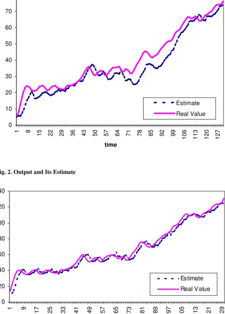
In figures 1, 2, and 3, the data that has been generated from the model are displayed along with the estimations that have been obtained via EKF. Also, the recursive estimates for the parameters can be seen in figures 4, 5 and 6. Figure 4 implies that the parameter “a” takes values between 0.45 and 0.65, which makes sense as a measure of marginal propensity to consume. The parameter “b”, on the other hand, can be viewed as being stable around 0.5 after a sharp drop in the first 10 periods. Finally, in figure 6, parameter “d” in the equation for government expenditure has been stable around 1, consistent with the random walk assumption. As a result, it will not be wrong to claim that the recursive estimates for the parameters are meaningful and the estimated state variables are very close to their simulated values.
5. Results
In this study, a simple ad-hoc Keynesian model has been employed to test the estimation power of Extended Kalman Filter, which is the appropriate methodology to be used in non-linear state space models. Although the model can be criticized for being too stylized, it is the first attempt to estimate a macroeconometric model for the Turkish economy using Extended Kalman Filter. The results obtained from the simulation exercise show that the estimated state variables are very close to the simulated series, and the recursive parameter estimates are fairly reasonable. These findings suggest that the estimation methodology that has been introduced in this study has the potential to be used in more complex and realistic models with real-time data applications.
References
Aliev, F. and Ozbek L. 1999. Evaluation of Convergence Rate in the Central Limit Theorem for the Kalman Filter. IEEE Trans. Automatic Control 44(10): 1905-1909.
Anderson, B. D. O. and. Moore, J.B. 1979. Optimal Filtering. Prentice Hall.
Bacchetta, P. and Gerlach, S. 1997. Consumption and Credit Constraints: International Evidence.
Journal of Monetary Economics 40(2): 207-238.
Chen, G., 1993. Approximate Kalman Filtering. World Scientific.
Chui, C. K. and Chen, G. 1991. Kalman Filtering with Real-time Applications. Springer Verlag. Durbin, J. and Koopman, S.J. 2001. Time Series Analysis by State Space Methods. Oxford University
Press.
Efe, M. and Ozbek, L. 1999. Fading Kalman Filter for Manoeuvring Target Tracking. Journal of the
Turkish Statistical Assocation 2(3): 193-206.
Grillenzoni, C. 1993. ARIMA Processes with ARIMA Parameters. Journal of Business and Economic
Statistics 11(2): 235-250.
Harvey, A. C. 1990. Forecasting, Structural Time Series Models and the Kalman Filter. Cambridge: Cambridge University Press.
Jazwinski, A. H. 1970. Stochastic Processes and Filtering Theory. Academic Press.
Ljung, L. and Söderström, T. 1983. Theory and Practice of Recursive Identification. Cambridge, Mass: MIT Press.
Ljungqvist L. and Sargent T. 2000. Recursive Macroeconomic Theory. MIT Press.
McKiernan, B. 1996. Consumption and the Credit Market. Economics Letters 51(1) (April): 83-88. Ozbek, L. 2000. Durum-Uzay Modelleri ve Kalman Filtresi. Gazi Ünv. Fen Bilimleri Ens. Dergisi 13(1):
113-126.
. 2001. Sistem Tanılamada Uyarlanır Kalman Süzgeci ve Sıcaklık Denetimi çin Bir Uygulama
Çalı ması. Galatasaray Ünv. Mühendislik Bilimleri Dergisi 1(2): 15-28.
Ozbek, L and Efe, M. 2000. Online Estimation of the State and the Parameters in Compartmental Models Using Extended Kalman Filter. In the book, Nonlinear Dynamics in the Life and Social Sciences. Editors: Sulis, W.H. and Trofimova, I. pp 262-274, IOS Press.
. 2003. An Adaptive Extended Kalman Filter with Application to Compartment Models.
Communication in Statistics-Simulation and Computation, forthcoming.
Reif, K. and Unbehauen, R. 1999. The Extended Kalman Filter as an Exponential Observer for Nonlinear Systems. IEEE Trans. Signal Processing 47(8): 2324-2328.
Reif, K., Gunther, S., Yaz, E. and Unbehauen, R. 1999. Stochastic Stability of the Discrete-Time Extended Kalman Filter. IEEE Transactions on Automatic Control 44(4): 714-728.
Tanizaki, H. 2000. Nonlinear and Non-Gaussian State-Space Modeling with Monte Carlo Techniques: A Survey and Comparative Study. Kobe University, Faculty of Economics Working Paper.
Fig. 1. Consumption and Its Estimate
Fig. 2. Output and Its Estimate
0 10 20 30 40 50 60 70 80 1 8 15 22 29 36 43 50 57 64 71 78 85 92 99 10 6 11 3 12 0 12 7 time Estimate Real Value 0 20 40 60 80 100 120 140 1 9 17 25 33 41 49 57 65 73 81 89 97 10 5 11 3 12 1 12 9 tim e Estimate Real Value
Fig. 3. Government Exp. and Its Estimate
Fig. 4. Parameter 'a'
0 10 20 30 40 50 60 1 8 15 22 29 36 43 50 57 64 71 78 85 92 99 10 6 11 3 12 0 12 7 time Estimate Real Value 0 0,1 0,2 0,3 0,4 0,5 0,6 0,7 1 8 15 22 29 36 43 50 57 64 71 78 85 92 99 10 6 11 3 12 0 12 7 time Parameter 'a'
Fig. 5. Parameter 'b' Fig. 6. Parameter 'd' 0 0,2 0,4 0,6 0,8 1 1,2 1,4 1 8 15 22 29 36 43 50 57 64 71 78 85 92 99 10 6 11 3 12 0 12 7 time Parameter 'd' 0 0,1 0,2 0,3 0,4 0,5 0,6 1 8 15 22 29 36 43 50 57 64 71 78 85 92 99 10 6 11 3 12 0 12 7 time Parameter 'b'