Discussions and Closures
Discussion of
“Critical Values for S¸en’s Trend Analysis”
by Richard H. McCuen
Eyüp S¸ işman, Ph.D.
Assistant Professor, School of Engineering and Natural Sciences, Civil En-gineering Dept., Istanbul Medipol Univ., Beykoz, Istanbul 34815, Turkey; Assistant Professor, Climate Change Researches Application and Research Center, Istanbul Medipol Univ., Beykoz, Istanbul 34815, Turkey (corre-sponding author). Email: [email protected]
Yavuz Selim Güçlü, Ph.D.
Associate Professor, Engineering and Natural Sciences Faculty, Istanbul Medeniyet Univ., Uskudar, Istanbul 34700, Turkey. Email: yavuzselim [email protected]
İsmail Dabanlı, Ph.D.
Associate Professor, School of Engineering and Natural Sciences, Civil En-gineering Dept., Istanbul Medipol Univ., Beykoz, Istanbul 34815, Turkey; Associate Professor, Climate Change Researches Application and Research Center, Istanbul Medipol Univ., Beykoz, Istanbul 34815, Turkey. Email: [email protected]
https://doi.org/10.1061/(ASCE)HE.1943-5584.0001708
It is well appreciated that the author of the original paper tried to avoid the qualitative subjectivity and proposed a quantitative ap-proach for trend identification in a given hydrometeorology time series. He considered that there are not quantitative publications on S¸ en’s innovative trend analysis (ITA) in the literature, which is not correct, because there are a few papers published on the quan-titative ITA trend estimation methodology (S¸ en 2017a,b). He also mentioned that trends are embedded into measurement data due to land cover or climate changes, which are systematic components in a given time series, but they are considered random variables, and therefore their identification needs probabilistic and statistical tests on the basis of some confidential limits, which are considered in practical applications as 5% or at the maximum 10%. Although trends may occur in temporal, spatial, or spatiotemporal spaces, the ITA method and original paper consider trends in time scale only. The purpose of this discussion is to support the explanations from the original paper on one hand, and on the other to indicate some of the invalid explanations and discussions throughout the text.
It is true that S¸ en did not provide any statistical mathematical quantitative test in the first publications concerning the ITA approach (S¸ en 2012,2014), but later on some quantitative method-ologies were presented (S¸ en 2017a,b). The author criticizes the statistical significance tests because of their significance level decision, but adaptation of 5% or 10% has become very common in the literature. The original paper considers the following three points as important:
1. The trend existence is modeled by the least-squares statistical approach.
2. An extensive simulation study through Monte Carlo tech-nique is carried out on the basis of different lengths (from 10 to 150) and a set of significance levels (0.1%, 1%, 2.5%, 5%, and 10%). The synthetic data generation is based on the serially independent stochastic structure with the normal probability distribution.
3. Some power of the proposed trend existence test is presented based on some empirical formulas based on the simulation study. The author’s criticism of the breakthrough point within the half-point of a time series is also very valid. He explains S¸ en’s (2012) ITA methodology clearly within four steps. Later in the text, he provided some actual and simulation annual flood data, but un-fortunately did not construct ITA graphs, which could stimulate better explanations.
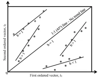
As for the“Proposed Test Statistic” section, the author has the right view that small deviations from the1∶1 line imply random var-iations without a trend component in the time series. Hence, the lack of trend will have a straight line with a slope of 45°, i.e.,1∶1. Hence he proposes one parameter model as in his Eq. (1). However, the statement “If the series does not include a trend, then b should be approximately 1.0” is very misleading because there may be par-allel lines to1∶1 lines in the upper or lower triangular areas of the ITA graph with trends, and these lines do not need to cross through the origin (Fig.1).
It is obvious from this graph that there may be trends with smaller or bigger slopes than 1 in increasing or decreasing manner. In the section of“Critical Values of Test Statistic,” b ¼ 1 is sug-gested as the population value, but as one can see from Fig.1, the null hypothesis cannot be accepted as a trendless case. Theb values greater than or less than 1 do not mean any critical value as for the trend existence or nonexistence. Although the author has made ex-tensive simulation study in the computer for depicting coefficients for the critical test, according to the preceding explanations, they are meaningless. In particular, the restrictive assumptions of sample length, normal probability distribution, and serial independence do not bring any additional dimension for the trend identification test. Subsequently, the critical values are described by some empiri-cal formulations [Eqs. (3)–(5)], but their scientific foundations are not clear in the original paper. There is no logical scientific basis for their suggestion, and therefore the reader is confused as to their validity. It is stated in this section again that an increasing trend is
Fig. 1. Various ITA trend components.
© ASCE 07019004-1 J. Hydrol. Eng.
J. Hydrol. Eng., 2020, 25(1): 07019004
expected such that the value ofb should be greater than 1.0, but as shown in Fig.1there are even decreasing trends withb < 1 or b > 1 in the lower triangular part of the ITA template. The use of upper or lower critical values in Table 2 are irrelevant.
In the“Power of Test” section, there are classical statistical sig-nificance suggestions that are available in the open literature. The word strength is used for the trend and hence there remains con-fusion whether it applies to the trend slope. Trend tests are depen-dent on the sample size, level of significance, and strength of the trend, but there is no mention about the probability density function (PDF) type, which is also important in such tests. Eq. (1) cannot be used for the power of the test statistics because it represents all the straight lines that cross through the origin, but there are cases where trends might not pass through the origin as is shown in Fig.1.
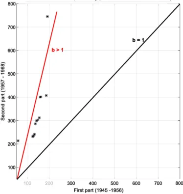
In the“Application of Test” section, the author unfortunately did not look for the data behaviors on the ITA template. Figs.2and3 are for annual maximum flood series records and simulation se-quences, respectively, because they are mentioned by the author. It is obvious that in Fig. 2there is a single monotonic trend withb > 1 in the annual maximum flood series in the Pond Creek catchment, whereas for the flood simulation values there are at least two trend components, one withb > 1 and the other with b < 1. It is rather surprising to notice that the simulation results do not resemble the actual annual maximum flood behavior. On the other hand, the author did not apply his critical values for the trend test at the Pond Creek watershed records.
The “Discussion and Implications” section contains some in-consistencies. For instance, the author mentions with an unfortunate
statement that a level of significance of 5% is often adapted regard-less of the importance of the problem; this should be avoided be-cause it cannot be considered in practical engineering applications because as a general tendency 5% or at the maximum 10% error bands are accepted in all water resources system studies. The author rightly pinpoints the fact that although the true break point is not known generally, its selection influences both the decision and the statistical power of the final decision.
After all that has been explained, there are recent publications that have given additional information about the quantification of the S¸ en (ITA) method (S¸ en 2017a,b;Mohorji et al. 2017).
References
Mohorji, A. M., Z. S¸ en, and M. Almazroui. 2017. “Trend analyses revision and global monthly temperature innovative multi-duration analysis.” Earth Syst. Environ. 1 (1): 9.https://doi.org/10.1007/s41748 -017-0014-x.
S¸ en, Z. 2012.“Innovative trend analysis methodology.” J. Hydrol. Eng. 17 (9): 1042–1046. https://doi.org/10.1061/(ASCE)HE.1943-5584 .0000556.
S¸ en, Z. 2014.“Trend identification simulation and application.” J. Hydrol. Eng. 19 (3): 635–642.https://doi.org/10.1061/(ASCE)HE.1943-5584 .0000811.
S¸ en, Z. 2017a. Innovative trend methodologies in science and engineering. New York: Springer.
S¸ en, Z. 2017b.“Innovative trend significance test and applications.” Theor. Appl. Climatol. 127 (3–4): 939–947.https://doi.org/10.1007/s00704-015 -1681-x.
Fig. 2. Pond Creek watershed annual maximum flood series, ITA template.
Fig. 3. Pond Creek watershed annual maximum flood simulations, ITA template.
© ASCE 07019004-2 J. Hydrol. Eng.
J. Hydrol. Eng., 2020, 25(1): 07019004