Low energy fixed clustering algorithm for wireless sensor networks

(1)

by Korhan Cengiz

Master degree, Electronics and Communications Engineering, Namik Kemal University

Submitted to the Graduate School of

Science and Engineering in partial fulfillment of the requirements for the degree of Electronics Engineering

Doctor of Philosophy

Kadir Has University 2016

(2)

(3)

Ben, Korhan Cengiz, bu doktora tezinde sunulan ¸calı¸smanın ¸sahsıma ait oldu˘gunu ve ba¸ska ¸calı¸smalardan yaptı˘gım alıntıların kaynaklarını kurallara uy-gun bi¸cimde tez i¸cerisinde belirtti˘gimi onaylıyorum.

(4)

ABSTRACT

LOW ENERGY FIXED CLUSTERING ALGORITHM

FOR WIRELESS SENSOR NETWORKS

Wireless sensor networks (WSNs) have become an important part of our lives as they can be used in vast application areas from disaster relief to health care. As a consequence, the life span and the energy consumption of a WSN has become a challenging research area. According to the existing studies, instead of using direct transmission or multi-hop routing, clustering can significantly reduce the energy consumption of sensor nodes and can prolong the lifetime of a WSN. In this thesis, low energy fixed clustering algorithm (LEFCA) and multi-hop low energy fixed clustering algorithm (M-LEFCA) are proposed for WSNs. With LEFCA, the clusters are constructed during the set-up phase. A sensor node which becomes a member of a cluster stays in the same cluster throughout the life span of the network. LEFCA not only improves the lifetime of the network, but also decreases the energy dissipation significantly. In addition, proposed M-LEFCA uses multi-hop intra cluster communication approach. It selects optimum forward neighbor cluster heads (CHs) as relay nodes (RNs). M-LEFCA aims to reduce energy dissipation and prolong network lifetime of LEFCA by combining clustering and multi-hop routing approaches.

(5)

¨

OZET

KABLOSUZ SENS ¨

OR A ˘

GLARI ˙IC

¸ ˙IN D ¨

US

¸ ¨

UK

ENERJ˙IL˙I SAB˙IT K ¨

UMELEME ALGOR˙ITMASI

Kablosuz sensör a˘gları afet yardımından sa˘glık hizmetlerine kadar bir¸cok uygulama alanında kullanılabildiklerinden ötürü hayatımızın önemli bir par¸cası olmu¸stur. Bunun sonucu olarak, kablosuz sensör a˘glarının ömrü ve enerji tüketimi ilgi ¸cekici bir ara¸stırma alanı haline gelmi¸stir. Mevcut ¸calı¸smalara göre, direkt haberle¸sme veya ¸cok-sekmeli yönlendirme yerine kümeleme, sensör dü˘gümlerinin enerji tüketimini önemli öl¸cüde azaltabilir ve kablosuz sensör a˘gının ömrünü uzatabilir. Bu tezde, kablosuz sensör a˘gları i¸cin dü¸sük enerjili sabit kümeleme algoritması (LEFCA) ve ¸cok-sekmeli dü¸sük enerjili sabit kümeleme algoritması (M-LEFCA) önerilmektedir. LEFCA ile, kümeler kurulum evresi esnasında in¸sa edilmektedir. Bir kümenin elemanı olan sensör dü˘gümü a˘gın ömrü boyunca aynı kümede kalmaktadır. LEFCA sadece a˘gın ömrünü uzatmamakta ayrıca enerji tüketimini de önemli öl¸cüde azaltmaktadır. Bununla beraber, tasarlanan M-LEFCA ¸cok-sekmeli kümeler arası haberle¸sme yakla¸sımını kullanmaktadır. Op-timum ileri yönlü kom¸su küme ba¸slarını aktarıcı dü˘güm olarak se¸cmektedir. M-LEFCA kümeleme ve ¸cok-sekmeli yönlendirme yakla¸sımını birle¸stirerek LEFCA’ nın enerji tüketimini azaltmayı ve a˘g ömrünü uzatmayı ama¸clamaktadır.

(6)

ACKNOWLEDGEMENTS

First of all, I express my sincere gratitude and respect to my advisor Dr. Tamer Da˘g for their encouragement, support and guidance. Furthermore, I would like to thank to the members of my PhD committee Dr. Serhat Erkü¸cük, Dr. Ay¸segül Tüysüz Erman, Dr. Erdal Panayırcı and Dr. M. Tolga Sakallı for their valuable comments, suggestions and their time spent on reviewing my thesis.

I would like to thank to the ”Tubitak Priority Areas Scholarship Pro-gramme (2211-C)” for its financial support to my Ph.D. thesis. I would like to thank to the department members of Electrical-Electronics Engineering of Trakya University and Dr. Eylem Erdo˘gan for their encouragement, support and enjoyable times we spent together and my deepest gratitude goes to my beloved parents, my brother and my aunt for their immeasurable dedication, faithful support and great encouragement.

(7)

(8)

LIST OF FIGURES

1.1 An example for voltage sensor . . . 1

1.2 Overview of sensor node hardware components . . . 4

1.3 An example for a WSN . . . 5

2.1 Direct Communication in WSNs . . . 14

2.2 Multi-Hop Routing in WSNs . . . 15

2.3 Clustering in WSNs . . . 16

3.1 The Overview of LEFCA Algorithm . . . 31

3.2 The Set-up Phase for LEFCA Algorithm . . . 32

3.3 CH Selection Phase for LEFCA Algorithm . . . 33

3.4 Determination of CHs by BS . . . 34

3.5 Cluster topologies for 5, 6, 9 and 10 clusters . . . 35

3.6 ADV Message Structure of LEFCA . . . 35

3.7 Collision Mechanism in CSMA . . . 37

3.8 Join-REQ Message Structure of LEFCA . . . 40

3.9 Example for CH Selection in LEFCA . . . 41

3.10 Time slot assignment for cluster members in a LEFCA cluster 42 3.11 Example of Time slot assignment for cluster members in cluster 2 of Fig. 3.9 . . . 42

3.12 Cluster Formation . . . 43

3.13 The Steady State Phase of LEFCA . . . 44

3.14 The LEFCA Round. Data transfers and changing of CHs if needed occur during the steady-state phase. . . 44

(12)

3.15 Narrow band signal. . . 45

3.16 Matched Filter . . . 49

3.17 CH changes in LEFCA . . . 52

3.18 Outside BS Situation . . . 54

4.1 CH Determination by BS . . . 58

4.2 CH ADV Message Structure of M-LEFCA . . . 58

4.3 Cluster Formation after Joining of Cluster Members . . . . 59

4.4 Multi-hop Relay Node Determination in M-LEFCA . . . . 60

4.5 RN Selection Notification Message Structure in M-LEFCA 60 4.6 Data Transmission in M-LEFCA . . . 61

5.1 Lifetime Performance of Random and Intelligent CH Selec-tion of LEFCA with regard to the Number of Clusters . . . 66

5.2 Number of Dead Nodes according to the di↵erent ThVs . . 67

5.3 Energy levels of the nodes . . . 68

5.4 Energy Map of the Network . . . 70

5.5 Round Number vs. Residual Energy . . . 72

5.6 Round Number vs. Number of Alive Nodes . . . 73

5.7 Round Number vs Total Data Transmitted to the BS . . . 75

5.8 Round Number vs. Number of Alive Nodes for 50 Nodes . 76 5.9 Round Number vs. Number of Alive Nodes for 200 Nodes . 77 5.10 Round Number vs. Number of Alive Nodes for Inside BS Situation . . . 79

5.11 Residual Energy Comparison of LEFCA and M-LEFCA . . 80

5.12 Round Number vs. Number of Alive Nodes for LEFCA and M-LEFCA . . . 81

(13)

5.13 Round Number vs Total Data Transmitted to the BS for LEFCA and M-LEFCA . . . 83

(14)

LIST OF TABLES

3.1 Determination of ThV . . . 56 5.1 Simulation Environment Parameters . . . 65 5.2 Network Lifetime Comparison . . . 74 5.3 Average Network Lifetime Comparison for Di↵erent Situations 78 5.4 Network Lifetime Comparison of LEFCA with M-LEFCA . 82

(15)

LIST OF ABBREVIATIONS

ADC analog-to-digital converter

WSN wireless sensor network

BS base station

CH cluster head

LEFCA low energy fixed clustering algorithm

M-LEFCA multi-hop low energy fixed clustering algorithm

RN relay node

LEACH low energy adaptive clustering hierarchy LEACH-F leach fixed clustering

ModLEACH modified leach

SEP stable election protocol

DEEC distributed energy-efficient clustering scheme PDA personal digital assistant

TDMA time division multiple access

ADV advertisement message

CSMA carrier sense multiple access

MAC medium access control

REQ request message

FDMA frequency division multiple access CDMA code division multiple access SDMA space division multiple access

(16)

DS-SS direct-sequence spread-spectrum FH-SS frequency-hopping spread-spectrum

PN pseudo noise

AM amplitude modulation

DSB double side band

SSB single side band

SNR signal-to-noise ratio

ThV threshold value

ICT information communication technology MACA multiple access collision avoidance

(17)

1. INTRODUCTION

A sensor is an equipment that senses and replies to particular kind of input from nature. An example for a sensor is shown in Fig. 1.1 [1]. The illustrated sensor measures voltage. The specific input that a sensor measures can be heat, motion, moisture, pressure, light, or many other environmental event. The output becomes a signal which is converted to a screen at the sensor position or transmitted electronically over a network for evaluating or further processing. A typical sensor should have following characteristics to provide the desired performance [2]:

Figure 1.1: An example for voltage sensor

• High Sensitivity: Sensitivity states how much the output of the device varies with unit change in input. For instance the voltage of a temperature

(18)

sensor changes by 1mV for every 1 C change in temperature thus, the sensitivity of the sensor becomes 1mV/ C.

• Linearity: The relation between input and output should be linear. • High Resolution: Resolution is the minimum alteration in the input that

the sensor can sense.

• Less Noise and Disturbance: Noise and disturbance should be mini-mized to obtain consistent measurements.

• Power saving: Power saving is very important to prolong the lifetime of a sensor node.

Sensors can be categorized based on the type of quantity they measure. The main kinds of sensors can be listed as below [3] - [6]:

• Acoustic and sound sensors: An acoustic sensor is a device that measures sound levels.

• Automotive sensors: These sensors are used in automotive industry. The three major areas of systems application for automotive sensors are pow-ertrain, chassis, and body.

• Chemical Sensors: A chemical sensor is a device that converts chemical information (composition, presence of a particular element or ion, concen-tration ...) into an analysable signal.

• Magnetic Sensors: Magnetic Sensors use the changes in magnetic field for their operations. Magnetic sensors can determine presence, direction and speed of a vehicle.

(19)

surface characteristics that support the information requirements for e↵ec-tive environmental management.

• Optical Sensors: Optical sensors transform light, or an alteration in light, into an electronic signal.

• Mechanical Sensors: Mechanical sensors measure mechinal quantities such as pressure, force, torque, velocity, mass and density.

• Thermal and Temperature sensors: A thermal sensor is a device that is specifically used to measure temperature.

• Proximity and Presences sensors: A proximity sensor is capable to sense the presences of close objects without any physical impact. It usually propagates electromagnetic radiations and detects the changes in reflected signal.

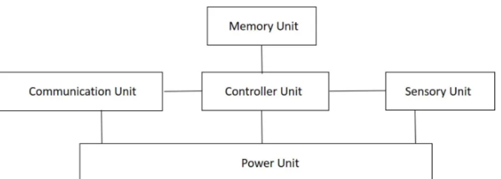
A typical wireless sensor node is composed of a sensory unit, a communi-cation unit, a power unit, a controller unit and a memory unit which is shown in Fig. 1.2. The sensory unit has a data acquisition component and ADC. The communication unit has a radio transceiver. The power unit is supported by a battery source. The controller unit is the core of a wireless sensor node. Controller unit gathers, processes data and decides when and where to send it. Memory unit is used to store sensor readings and packets from other nodes [7].

Typically, wireless sensor nodes can only be equipped with restricted en-ergy sources. The node remains active as long as the battery is not dead and hence power savings is usually a crucial criterion in this domain of applications. Energy consumption can occur in sensing, data processing and communications

(20)

Figure 1.2: Overview of sensor node hardware components

components. The sensing and data processing components consume less than 1mW of energy. The communication component on the other hand is considered as the most energy consuming part, as a result it has a significant impact on network lifetime.

1.1. Wireless Sensor Networks (WSNs)

WSNs compose of numerous sensor nodes distributed over a geographical area with predefined positions or random deployment. By sensing the environ-mental events within their respective ranges sensor nodes collect data of interest and communicate the data through the nodes until the data finally arrives at the base-stations (BSs) for final processing which is shown in Fig. 1.3 [8].

WSNs are used in a vast array of applications which may require fixed monitoring and detection of specific events such as environmental applications, military applications, patient monitoring, disaster relief, and smart home, fa-cility management, precision agriculture, logistics, telematics and smart city systems [9].

(21)

Figure 1.3: An example for a WSN

Energy-efficient communication and routing protocols can help an increased network lifetime for WSNs.

Routing is described as the mechanism of determining a path between the source and the destination node upon request of message transmission from the source node. In WSNs, the network layer is mostly used to implement the routing of data messages.

Routing in WSNs is very challenging due to the intrinsic characteristics that distinguish these networks from other wireless networks, such as mobile ad hoc networks or cellular networks. Due to the unique characteristics and

(22)

properties of a WSN, the existing routing protocols developed for wireless ad hoc networks cannot be directly applied to WSNs. The design of a routing protocol for WSNs has to consider the unreliability of the wireless channel, the potential dynamic changes in the network topology, as well as the limited processing, storage, bandwidth, and energy capacities of the WSN nodes. Therefore, special approaches are needed to guarantee efficient routing amongst the nodes of a WSN [10].

1.1.1. WSN Performance Metrics

The performance of WSNs is measured based on quantifiable parameters called performance metrics. The metrics however vary according to the need and the nature of WSNs. Throughput, latency, overhead, energy-efficiency, scalabil-ity, network lifetime, can be considered as common performance metrics for WSNs [11, 12].

The throughput represents the e↵ective network capacity. It can be de-fined as the total count of bits which are delivered at the destination in a given period of time successfully. As the throughput of the network increases, the performance of the system increases. Especially imaging WSN systems require significant throughput because nodes produce high-speed data streams, such as a camera sensor node transmits images for target tracking, often require high throughput. Thus, specific WSN applications require throughput maximization and throughput guarantees. In order to enhance the resource efficiency, further-more, the throughput of WSN should often be maximized.

(23)

Latency is a measure of the average delay between transmitting a message and receiving it at the base station. Latency can be determined by calculating the total time elapsed to perform an action by the sensor nodes.

Overhead is the amount of extra information embedded into the sensor data in order to accomplish tasks required by the network.

Energy efficiency of a WSN can be found by calculating energy consump-tion in the network. Energy dissipaconsump-tion of each sensor can be described as the normalized total amount of energy used in receiving or sending data.

The ability to sustain performance characteristics regardless of the size of the network is named as scalability. As the size of the network expands, or the number of nodes increases, the routing protocol should adapt to the changes and provide appropriate performance. WSNs may include too much nodes, thus, some nodes can obtain limited information about network topology. Therefore, fully distributed protocols need to be developed to ensure scalability.

Network lifetime metric for WSNs is application dependent. Various met-rics for network lifetime have been proposed for varied scenarios in WSNs. Com-mon lifetime metrics are listed below [13]:

• The time until the last sensor node dies [14] - [17]: This definition indicates that a WSN is functional until the death of the last sensor node in the WSN.

(24)

• The time of the first node failure [18] - [21]: The first node which is failed in the WSN is used for defining the network lifetime. The dead node is generally called a critical node. If all the nodes have equal importance, this metric is not very useful for WSNs.

• The number of alive nodes [22]: The number of alive nodes is used as a measurement for network lifetime. Much number of alive nodes corre-sponds to longer network lifetime. It is commonly held lifetime metric for homogeneous WSNs.

• The time of an exact fraction of living nodes [23] - [25]: The network lifetime is identified by the fraction of living nodes as a function of time. The network is living while the fraction of surviving nodes still have energy above a target ThV.

• The lifetime in terms of packet delivery rate [23, 26]: This definition eval-uates the lifetime depending on the time until the packet delivery ratio drops severely. The network disconnectivity occurs at time t when the packet delivery ratio falls below the ThV.

• The number of nodes that stay connected to the BS [22]: The surviving rate of the network is measured according to the number of nodes remaining connected to the BS. The number of nodes that have to remain connected to the BS can be predetermined.

In addition to the above lifetime definitions, some applications use the approaches mentioned below:

(25)

• The time to the first loss of coverage [28].

• The time until the first cluster head (CH) is drained of its energy [29]. • The time each target is covered by at least one node [30].

• The time the whole area is covered by at least one node [31].

1.2. Motivation and Contributions

In this thesis, Low Energy Fixed Clustering Algorithm (LEFCA) which aims to use fixed clustering and CH determination via BS approaches together is proposed. In addition to existing algorithms, LEFCA uses intelligent CH determination mechanism which tries to elect the nodes that are almost at the center of their associated clusters at the beginning of the algorithm instead of determining them randomly. The formed clusters stay fixed for the entire network lifetime. A novelty that, LEFCA introduces a threshold based CH change mechanism. It aims to abuse the energies of the CHs before electing a new CH. The exploitation of CHs is not proposed in any of the existing algorithms in the literature. The results of LEFCA indicate that significant energy savings, lifetime improvements and throughput maximization can be obtained.

In this thesis, in addition to LEFCA, Multi-Hop Low Energy Fixed Clus-tering Algorithm (M-LEFCA) which combines clusClus-tering and multi-hop routing is proposed. M-LEFCA uses a fixed clustering approach. While the clusters who are far away from the BS use relay nodes (RNs) to transmit the collected data, neighbour clusters to the BS transmit their collected data directly to the BS. M-LEFCA is composed of two phases. In the set-up phase the CHs are elected,

(26)

the clusters are formed and RNs are determined. In the steady-state phase data collected from each cluster is transmitted to the BS by using RNs or directly. CH and RN changes also occur in the steady-state phase if needed.

1.3. Organization

The thesis is organized as follows;

• Chapter 2 explains communication in WSNs in terms of direct communi-cation, multi-hop routing and clustering.

• Chapter 3 explains the architecture of the proposed LEFCA protocol. LEFCA starts with the set-up phase where cluster formation occurs and continues with steady-state phase in which data transmission is performed and cluster head (CH) change decision is analyzed.

• Chapter 4 presents the multi-hop LEFCA (M-LEFCA) which uses cluster head nodes as relay nodes to transmit collected data and decrease commu-nication distances of cluster head nodes between base station.

• In Chapter 5, simulation environment and parameters of LEFCA and M-LEFCA are presented. The performance metrics of M-LEFCA and M-M-LEFCA are compared with LEACH, LEACH-F, MODLEACH, SEP and DEEC by realizing the simulations.

(27)

2. COMMUNICATION IN WSNs

Routing in WSNs di↵ers from traditional routing in fixed networks in sev-eral ways. There is no infrastructure, wireless links are uncertain, sensor nodes can fail. In WSNs, it is impossible to design a global addressing approach for the placement of sensor nodes. Consequently, traditional IP-based protocols cannot be applied to WSNs. In contrary to traditional networks nearly all applications of WSNs need the traffic of sensed data from multiple resources to a specific BS. Sensor nodes are restricted in terms of transmission power, processing capacity and memory and accordingly need efficient resource administration. By the rea-son of these di↵erences, various algorithms are designed for the issue of routing messages in WSNs. These routing approaches consider the characteristics of sensor nodes associated with the application and architecture necessities.

The design of routing algorithms in WSNs is a↵ected by many factors. These factors constitute challenges that must be overcome before efficient com-munication can be achieved in WSNs. Some of the routing challenges can be listed as [7, 32]:

• Energy Consumption: Energy consumption is considered one of the major concerns in routing protocols for WSNs. Nodes can drain their limited energy resources while transmitting information in a wireless environment. While forming their routing tables, nodes consume energy by exchanging messages with their neighbors.

(28)

• Node Mobility: In some cases, nodes are not stationary. Node mobility causes to happen changes in the neighborhood relations; nodes get out of range of their neighbors.

• Node Deployment: Node deployment in WSNs can be either deterministic or random, which is dependent on the required application. In random deployment, nodes may be placed randomly in arbitrary positions. The network topology can change dynamically thus, nodes may not be aware of the network topology. Therefore routing protocol should provide topology information.

• Robustness: Routing in WSNs is based on the sensor nodes to transmit data in a multi-hop style. Hence, routing protocols operate on these nodes instead of assigned routers. Thus, routing protocols should provide robust-ness to sensor node failures.

• Application: The type of application is also important for the design of routing protocols. In case of monitoring applications, static routes can be used again to sustain efficient delivery of the measurements. On the other hand, in event-based applications, since some of the nodes put their mode to sleep mode, when an event occurs, routes should be built to transmit the event information on time.

In general, the routing protocols for WSNs can be categorized as direct communication, multi-hop routing and clustering.

(29)

2.1. Direct Communication

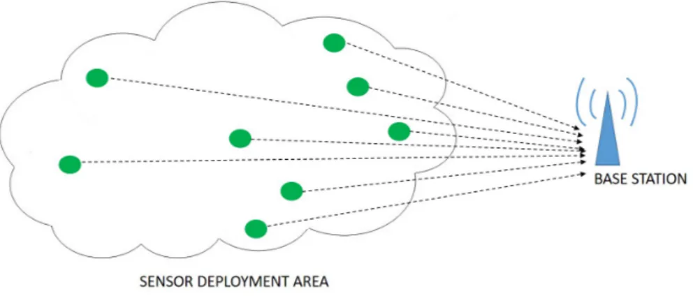
This is the simplest routing protocol which consists of only BS and sensor nodes. The sensor nodes act as senders and BS serves as the destination node to all the other sensor nodes in the network [33, 34]. Each sensor node collects and transmits the data directly to the BS in direct transmission as shown in Fig. 2.1. The communication between the sensor nodes and BS is direct without any intermediate nodes. The nodes only become active during the data transmission to the BS. Consequently, in direct transmission, sensor nodes do not consume energy to receive packets from the other nodes, but they will spend their battery resources on transmitting messages to the BS.

BS is the entity where information is required. There are three types of base stations: First type, it can belong to the sensor network. Second type can be located at outside of the sensor field. For this case, it can be an actual device such as a Personal Digital Assistant (PDA) used to communicate with the sensor nodes. Third type is a gateway to another larger network such as the Internet.

If the BS is far away from the sensor nodes, the batteries of the nodes will be drained quickly. Thus, direct transmission is not appropriate for WSNs which are deployed over large areas.

(30)

Figure 2.1: Direct Communication in WSNs

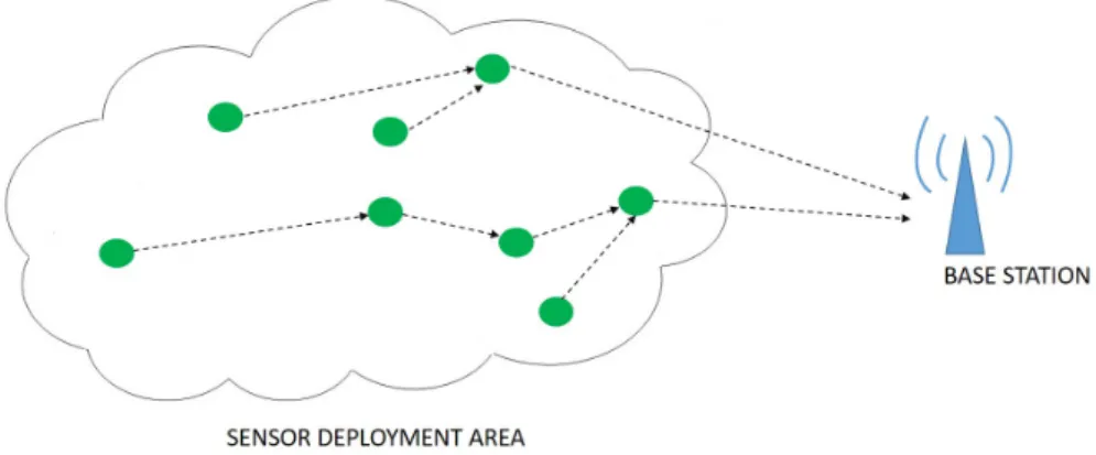
2.2. Multi-hop Routing

In multi-hop routing, several multi-hop paths are used to satisfy the net-work connectivity as illustrated in Fig. 2.2. Each node acts two di↵erent and supplementary roles in multi-hop routing [7]: data originator where each sensor node collects data from the environment via sensors and the collected data are processed and sent to neighbour sensor nodes for multi-hop transmission to the BS, data router in which each sensor is used as relay node for its neighbours.

In a large network, multi-hop communication becomes necessary because nodes relay the packets sent by their neighbors to the BS. Therefore, the sensor node is liable for collecting the data transmitted by its neighbors and forwarding these data to one of its neighbors in compliance with the routing decisions.

Nodes closer to the BS consume their energy rapidly as they have more data to process coming from the downstream nodes [10]. Due to the heavy load

(31)

on the relaying nodes, multi-hop routing may not be suitable for dense WSNs.

Figure 2.2: Multi-Hop Routing in WSNs

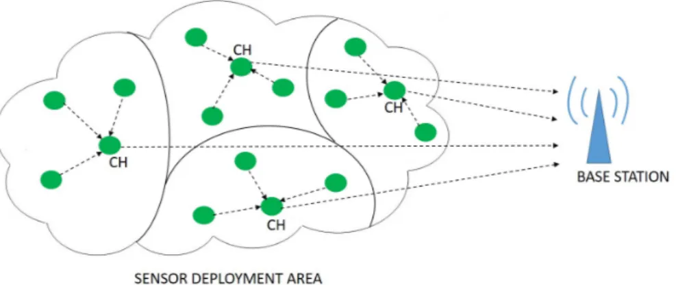
2.3. Clustering

In clustering, nodes are arranged into clusters that communicate through a cluster head (CH). The CHs gather data from their associated members, ag-gregate the data and transmit them to the BS which is shown in Fig. 2.3. By this way, the average transmission distance of the nodes to the base station de-creases. The sensed data is received by the BS within just two hops. Thus, clustering provides significant energy savings in WSNs.

Some of the major clustering protocols are described below.

2.3.1. LEACH

LEACH [16, 29, 35] is a well-known, simple and efficient round based adaptive clustering routing protocol for WSNs. In LEACH, clusters are formed

(32)

Figure 2.3: Clustering in WSNs

randomly in an adaptive and self-organized way. The nodes in the network form clusters without any help from any external agent or a certain node in the network.

In LEACH protocol, the time is divided into frames called a round. Each round consists of two phases. The first phase is the set-up phase where CHs are determined and clusters are formed. The second phase is on data collection and transmission and is called as the steady-state phase. In the set-up phase, the CHs are elected based on a probability function. In the CH election process, a predetermined fraction of nodes elect themselves as CHs. The nodes in the network choose a random number between 0 and 1 and this number is compared with threshold limit. If this random number is less than the threshold value, T (n), the node becomes the CH for the current round. The threshold value is calculated based on following equation:

T (n) = p

(33)

where G is the set of nodes that are not selected as a CH in the last (1/p) rounds, p is the desired percentage to become a CH, r is the current round.

This probability function is performed in such a way that in a specific number of rounds each node is elected as CH for once and hence the energy con-sumption is fairly distributed over the entire network. After the set-up phase of the round, where the CHs are elected, each CH announces its identity to the other nodes and the remaining nodes, choose a suitable (nearest) CH for themselves and announce this decision to the related CH and thus the clus-ters are formed and the network enclus-ters into the steady-state operation i.e data transmission. Each CH creates a TDMA schedule for its cluster to organize the communication among cluster members. When the non CH nodes receive the TDMA schedule, they send their data to the CH once per frame during their allocated transmission TDMA slots. This allows the radio components of each non CH node to enter the sleep mode at all times except during its transmission time, thus minimizing the energy dissipated in the individual sen-sors. The CHs then send the collected data to the BS and one round completes. With the next round, the above process repeats. To prevent the interference of the transmissions which occur in di↵erent clusters at the same time, LEACH uses di↵erent CDMA codes. CHs randomly choose a unique code from a list of spreading codes. The CHs filter all received energy using this spreading code. Consequently, the radio signals of the neighboring clusters are filtered out hence interference of the transmission of the nodes is minimized.

(34)

based on self-configuring network principle. The nodes are self-organized to perform related network tasks such as electing themselves as CHs, forming clus-ters, etc. All the sensor nodes are CH candidates and all of them are assumed to have access to the BS.

LEACH causes a balanced energy dissipation of sensor nodes in the network when compared with direct transmission and multi-hop routing. Thus with LEACH the entire network is sensed during the lifetime of the network.

On the other hand, there are several disadvantages of the LEACH protocol. The clusters and CHs are chosen randomly. Thus, inefficient cluster formations and unbalanced cluster sizes across the network is highly probable. Due to the random nature of CH election process, sensor nodes which are far away from the BS can become CHs causing more energy consumption. Remote nodes tend to die earlier. Cluster topologies and CHs change every round, at the cost of extra overhead and energy dissipation.

2.3.2. LEACH Variants

Numerous studies are designed to improve the performance of LEACH. Many of them aim to change the CH selection process of LEACH to obtain energy-efficiency. The work in [36] - [43] can be considered in this group. CHs and cluster formations are changed in each round of LEACH. This structure of LEACH causes to consume large amount of energy. Due to this restriction, CH selection is managed adaptively according to the energy reserve

(35)

of local active nodes in [36]. Unlike LEACH, this approach is a distributed self-organizing scheme without any centric control and it has higher tolerance than LEACH to on-o↵ topology changes. The adaptiveness of this approach makes significant reduction in communication-related energy dissipation.

Time-based CH selection for LEACH (TB-LEACH) is presented in [37]. TB-LEACH only modifies the CH election process of the LEACH to form uni-form cluster pieces. The competition for CHs depends on a random time interval in TB-LEACH. To become a new CH, a node has to have shortest time inter-val inter-value. The number of CHs is controlled with a counter. After the election of CHs, the remaining phases are same as LEACH. TB-LEACH has significant system lifetime values and better energy-efficiency than LEACH.

Advanced LEACH (ALEACH) is proposed in [38]. ALEACH presents a new CH election algorithm which provides selecting the best suited node for CH. For each round, authors contrive a new technique to select the most energy efficient nodes as CHs to reduce the death rate of the nodes. According to the results, ALEACH provides development in terms of network lifetime and energy efficiency.

Stable Cluster Head Election (SCHE) [39] enhances the CH election of LEACH to obtain the optimal probability of becoming a CH. According to several mathematical derivations of energy function in LEACH, authors find an optimal probability value for being CH. Simulations show that, this algo-rithm reduces significant amount of communication energy when compared with

(36)

LEACH.

Leader Election with Load Balancing Energy (LELE) is introduced in [40]. LELE compares the remaining energy and distance of a node with its neighbors to determine it as a CH. The homogeneous distribution of CHs is proposed in this protocol. The probability of being CH varies correlative with the di↵erence of the energy level of one node with its neighbors. It achieves better performance than LEACH in terms of energy-efficiency.

To solve the variability of the number of CHs problem in LEACH, authors develop Two Step Cluster Head Selection (TSCHS) in [41]. It uses two stages: temporary CH election stage and optimal CH election stage which is realized by using the current energy and distances to the BS of the temporary CHs to select CHs. Consequently, unlike LEACH, the number of CHs is changed and the network operates with the optimal number of clusters. TSCHS prolongs the lifetime and balances the energy wastage of the entire network. Optimal election of a CH is efficient in decreasing energy dissipation of the nodes and thus increases lifespan of the network.

Optimal CH selection algorithm which does not need to know the location information of the nodes is developed in [42]. The proposed algorithm works based on two parameters: the energy levels of the nodes and number of neighbors of the nodes. The algorithm also takes mobility of the nodes into consideration. The nodes may enter a new cluster when they move and the new CH is should be selected by moving nodes to provide energy-efficiency. After the simulations,

(37)

it is proved that, the remaining energy of the nodes is more than LEACH.

[43] labels the nodes as far and near nodes according to the distances to the BS. Then, proposed protocol forms singular clusters near the BS and multi clusters away from the BS using Greedy K-means algorithm. Proposed protocol provides significant life span improvement compared to LEACH.

LEACH-C [35] is derived from LEACH and needs the coordina-tion of the BS to select CHs. Some of the studies [45] - [47] in literature also aspire to develop the performance of LEACH-C by using some optimizations.

LEACH-CE [44] performs the same process as LEACH-C at appropriate time intervals. [45] proposes LEACH-Completely Controlled by Base-station (LEACH-CCB) that enhances LEACH-CE and presents two techniques: short circuiting dense communications of the nodes with base station and putting the specific percent of nodes into sleep mode for every round. This improved approach provides better network lifetime than LEACH-CE. LEACH-DC [46] uses CH candidates to determine the best CH in the WSN. LEACH-DC provides significant energy balance in WSN.

A novel cluster-head selection algorithm which uses the minimum mean distance between sensor nodes as a selection parameter for WSNs is presented in [47]. Proposed Low Energy Minimum Mean-Distance Algorithm (LEMMA) considers minimum mean distance between all the sensor nodes to reduce the energy usage of the non-cluster head nodes. However, in this protocol, the

(38)

position information knowledge of all sensor nodes should be known. Each sensor node sends its location information to the BS. Then BS calculates and sorts the mean distances of the sensor nodes. According to these distances BS constitutes CHs and clusters. According to results, LEMMA enhances the performance of LEACH in terms of throughput and network lifetime.

Modified LEACH (ModLEACH) [48] includes an efficient CH replacement scheme and dual transmitting power levels. The amplification energy is set to be the same for all kinds of transmissions in LEACH. But with ModLEACH, low energy level is used for intra cluster communications. Multi power levels are used to reduce the packet drop ratio, collisions and interference from other signals. When a node becomes a CH, the routing protocol in ModLEACH informs it to use high power amplification and when a node becomes a regular cluster member, the mode of that node becomes low level power amplification mode. Threshold based CH changing mechanism is used in ModLEACH to provide more efficient CH replacement. If the energy of the existing CH is higher than the threshold it continues to act as a CH, if not a new CH for that cluster is elected and the cluster is formed again.

While many homogeneous LEACH variants have been developed as de-scribed above, there are also heterogeneous cluster based WSN rout-ing protocols. Stable Election Protocol (SEP) [49] is a successful protocol for WSNs and contains advanced nodes which are fitted with extra energy re-sources. SEP uses a weighted election probability based approach to determine CHs according to the remaining energy of each node. In SEP, m corresponds

(39)

to fraction of the advanced nodes which are fitted with a times more energy than the normal nodes. As a consequence, the total initial energy of the WSN is increased by 1 + a.m times. The additional energy of the advanced nodes forces them to be elected as CHs. Each node is informed the total energy of the nodes in order to adjust its election probability to become a CH according to its residual energy. Two di↵erent weighted probabilities and thresholds are derived for normal and advanced nodes in SEP. The remaining energy values of normal and advanced nodes are transmitted to the CHs while members send data. The remaining energy values of the nodes are delivered to the BS via CHs. BS pe-riodically checks the heterogeneity in the network and broadcasts the updated weighted probabilities to the CHs according to the threshold. Finally, these updated weighted probabilities are transmitted to the members by CHs. The results of the simulations of the SEP show that, SEP provides significant en-ergy savings, lifetime gains and throughput improvement when compared with LEACH for both homogeneous and heterogeneous scenarios.

Distributed Energy-Efficient Clustering Scheme (DEEC) [50] is another heterogeneous and distributed clustering protocol where the cluster heads are elected by a probability based on the ratio between residual energy of each node and the average energy of the network. The nodes which have high residual en-ergy are more probable to become CHs. The epoch denoted by nicorresponds to number of rounds for node si to become CH. In homogenous networks, LEACH and many LEACH variants assume that the rotating epoch ni is same for all the nodes in the network. This causes to drain the battery of the low energy nodes more quickly than the high energy nodes. Therefore, di↵erent values for ni are

(40)

selected according to the residual energy of node si at round r in DEEC. The adaptive approach of DEEC provides for controlling the power dissipation of the nodes to accomplish the energy-efficiency objective of WSNs. In DEEC, there are advanced and normal nodes. m is the fraction of the advanced nodes and these nodes have a times more energy than the normal nodes. The preliminary energy of the nodes is randomly distributed between [E0, E0(1 + amax)] where E0 is the lower bound and amax determines the value of the maximal energy. Therefore, DEEC network has am times more energy and virtually am more nodes. The results of the simulations of DEEC protocol indicate that, DEEC prolongs the time of first node death when compared with LEACH variants and SEP in heterogeneous networks.

Efficient network partition algorithm is proposed to provide better energy saving performance than LEACH in [51]. Proposed algorithm splits the network into optimum segments and later picks the node with maximum energy as the CH for each segment by the use of the centralized calculations is suggested in this study. The results demonstrate that, pLEACH provides improvement in energy dissipation and network lifetime.

Considering the remaining energy of the nodes in the WSN to select the CH has become widely used and classical approach. [52] - [58] try to improve the performance of LEACH by using this way.

The remaining energy of the nodes is considered to select CHs in [52]. By this way, the proposed protocol aims to equalize energy dissipation distribution

(41)

in whole network. It also allows the neighbors of the BS to transmit their information directly to the BS. It prolongs the network lifetime efficiently when compared with LEACH.

Improved LEACH (I-LEACH) [53] considers residual energy of the nodes to select cluster heads and it tries to distribute CHs more efficiently than LEACH. The uniform distribution of the nodes is provided by using fixed locations. Node heterogeneity of I-LEACH protocol provides significant energy savings and life-time improvement when compared with LEACH.

Authors in [54] propose Universal LEACH (U-LEACH) algorithm to obtain additional energy savings. U-LEACH determines CHs according to their initial and current energy levels. It forms chains in each cluster to improve energy-efficiency. The nodes are aligned according to the distances to the BS in each chain for data transmission. It provides significant energy savings according to the LEACH.

The remaining energy of the nodes is considered to select new CH in the next round in [55]. Each existing CH receives the current energy of its members while it is collecting sensed data from its members. Then it forms a table which contains the IDs of the members and their remaining energies. Existing CH designates the node having the maximum energy to become new CH for next round according to this table. It considerably extends network lifetime when compared to LEACH.

(42)

[56] uses both remanent energy of the nodes and their distances to the BS for CH selection. A threshold value is also determined to start data transmission process of the nodes for providing more energy savings. The sensor field is divided into 4 quadrants. If a node is situated in the same quadrant of BS it has more chance to become a CH. Proposed protocol provides significant energy efficiency however, it needs position information of all the sensors in the WSN and this brings additional power consumption.

Authors in [57] present an unequal CH election mechanism algorithm. To extend the network lifespan, the residual energy values of the nodes should be calculated. This can be achieved by modifying the threshold equation of the LEACH. After this modification, each node has di↵erent threshold in comparison with a random number. As a result, the nodes which have high energy level get greater probability to be chosen as CHs. Simulations substantiate that the designed approach has higher energy-efficiency and can perform better network lifetime.

Far-Zone LEACH (FZ-LEACH) [58] forms a far-zone where the threshold value of residual energies of sensors is lower than a threshold. A zone head (ZH) is selected in this far-zone to collect data from other members. There is also ZH rotation in the far-zone. In LEACH, the desired number of clusters is determined by using analyzes and test simulations.

In LEACH optimum number of clusters is shown to be equal to five percent of the number of sensor nodes in the network. However, situations such as the

(43)

inside BS and di↵erent positions of BS are not considered. In some studies, [59] - [62], authors aim to enhance the desired number of clusters to provide better energy-efficiency performance.

Authors in [59], aim to optimize jointly the desired number of CHs and the spreading factor to extend the network lifetime of LEACH. According to the results, each number of desired CHs requires to be optimized separately for the corresponding additional spreading needed for minimizing the inter cluster interference.

In [60], LEACH-Balanced (LEACH-B) is developed. LEACH-B modifies the number of CHs in the network according to the remaining energy of the nodes. Consequently, the number of CHs becomes fixed.

The joint modification of optimum number of cluster heads and consid-ering the remaining energy of the nodes while electing a new CH are realized in [61]. A generalized mathematical expression is obtained to reach optimum clustering probability which includes three network parameters: average dis-tance between sensor field and the BS, area of the sensor field and the number of nodes distributed onto the field in the proposed algorithm. The proposed algorithm provides significant network lifetime improvements.

The relative distance between the nodes and BS, and the round number are parameters for improvement function which is discussed in [62] to improve existing LEACH algorithm. In this study, the number of CHs is managed by

(44)

modifying the threshold value used in LEACH. This modification provides the symmetrical threshold value distribution and it extends network lifetime signif-icantly compared with LEACH.

The optimization in threshold function and probabilistic CH elec-tion of LEACH is studied in the literature such as [63, 64]. The threshold function of the nodes in existing LEACH algorithm is considered to enhance three properties: the energy of each node, the duration of the CHs and the dis-tances between nodes and the BS in [63]. The simulation results prove that, the proposed improvement of LEACH outperforms LEACH in terms of network life span and energy-efficiency.

[64] aims to design efficient CH selection mechanism besides, objects to minimize the number of CHs by modifying the threshold expression of existing LEACH algorithm. Results prove that, the designed mechanism significantly decreases the energy consumption and prolongs lifetime of the network.

Instead of using di↵erent number of clusters for each round, using fixed number of clusters is also aimed to reduce the network overhead of LEACH in [35, 65, 66]. With LEACH Fixed Clustering (LEACH-F) [35], once the clus-ters are formed, there is no need to initiate the set-up phase repeatedly at the beginning of each round. The clusters are formed using a centralized cluster formation algorithm. They are formed once and fixed. The CH role is rotated between the nodes belonging to a cluster. During the set-up phase, each node transmits location information and energy level to the BS. Then the BS

(45)

com-putes the average node energy based on this information. The nodes which have energy under this average value do not become CHs for upcoming round. The top k nodes with maximum energy levels are determined to become CHs for the next round. When the optimal CHs and associated clusters are found, the BS sends a message back to all members in the network. This message contains the CH-ID for each node. If ID of a node matches this CH-ID, the CH role is taken by that node. If not, the node designates its TDMA slot for sending its packet and starts to sleep until data transmission. Note that, the CH selection is realized in order according to the CH-ID list. The first node listed in the cluster undertakes the CH role for the 1st round, the following node is found in that cluster list is selected CH for the 2nd round. Thus, the nodes are aware of when they become CHs and when they are normal members. The data transmission mechanisms of LEACH-F is same as in LEACH.

LEACH-IMP [65] uses constant CHs instead of rotation of CHs as in LEACH. Proposed protocol works generally in two phases. In the first phase, the nodes are homogenized according to divided grids. In the second phase, for each divided region, one CH is selected according to its optimal position in the cluster. This algorithm uses position information thus it can consume additional energy to overcome this determination. However, the homogeneous distribution provides more energy savings than LEACH.

[66] also presents dynamic round time based LEACH-F in which round time is designated based on the current energy levels of the nodes. The results demonstrate that dynamic round time based LEACH-F provides significant

(46)

en-ergy savings and lifetime enhancement when compared with LEACH.

Combination of multi-hop routing with clustering tries to enhance the performance of LEACH in [67]. Instead of direct transmission multi-hop routing in inter-cluster communication between CHs and BS is used. In this al-gorithm, when the cluster formations occur, CHs constitute a multi-hop routing backbone. They also enhance collision avoidance mechanism to prevent colli-sions. The simulations illustrate that, proposed algorithm provides significant energy gains when compared with LEACH.

(47)

3. THE LOW ENERGY FIXED CLUSTERING

ALGORITHM (LEFCA)

In this chapter, the proposed low energy fixed clustering algorithm (LEFCA) which includes set-up phase and steady-state phase is described in detail.

The proposed LEFCA algorithm uses the clustering approach by partition-ing the nodes into clusters. However, in this approach the clusters remain fixed throughout the entire lifespan of the WSN. In this manner, significant energy savings can be achieved. For each cluster, a CH is responsible for collecting and delivering the sensed data to the BS.

LEFCA algorithm is divided into an initial set-up phase where the clusters are determined and repeating LEFCA rounds where data is collected from the sensor deployment area by the CHs to be processed by the BS which is shown in Fig. 3.1. In each LEFCA round, existing CHs can be changed according to a threshold value, however clusters remain fixed for the entire WSN lifetime.

Figure 3.1: The Overview of LEFCA Algorithm

(48)

mech-anism performed by the BS. When the CHs are determined, the cluster forma-tion can start. In the steady-state phase of LEFCA, data transmission starts. During the steady-state phase, at the end of each round, the CH changing mech-anism is realized if needed. The following subsections describe the phases and its components of the LEFCA algorithm.

3.1. Set-Up Phase of LEFCA

After the deployment of the sensors, the LEFCA algorithm initiates with the set-up phase. The steps of the set-up phase are illustrated in Fig. 3.2. Some of the deployed sensor nodes are selected as CHs via the BS. A CH node is responsible for setting up the cluster by broadcasting its identity so that neighbor nodes join its cluster. When the members of a cluster are determined, the CH sets up and announces the TDMA schedule for the member nodes which denotes the corresponding time frames of data transmission for the cluster members. This phase starts with intelligent CH selection mechanism.

Figure 3.2: The Set-up Phase for LEFCA Algorithm

3.1.1. CH Selection Phase

Instead of selecting the CHs randomly, the intelligent CH determination mechanism is developed for LEFCA. Random selection of CH nodes provides

(49)

each node to have equal chance to become a CH at the beginning of each round. This mechanism reduces network costs because there is no need to use transmis-sion of position information to the BS. On the other hand, it may lead into some critical problems. CHs may be distributed unevenly throughout the network. Remote nodes can be selected as CHs resulting in significant energy dissipation and a shorter lifetime.

To annihilate these deficiencies, the intelligent CH selection mechanism is developed for LEFCA. The steps of CH selection is shown in Fig. 3.3. In intelligent CH selection mechanism, the BS broadcasts a position information request message to the WSN. When sensor nodes receive this message, each sensor node sends its position information to the BS. The transmission of the position information causes energy consumption by the nodes, however it is realized only once as the clusters will be fixed afterwards. After the transmission of the position information, the BS selects the CHs that are at the centre of each cluster. The number of clusters is determined according to the optimum cluster number for a WSN.

Figure 3.3: CH Selection Phase for LEFCA Algorithm

The BS selects 4, 8, 12 and 16 as CHs and notify them about the decision as shown in Fig. 3.4. The remaining nodes are not aware of their cluster membership yet.

(50)

Figure 3.4: Determination of CHs by BS

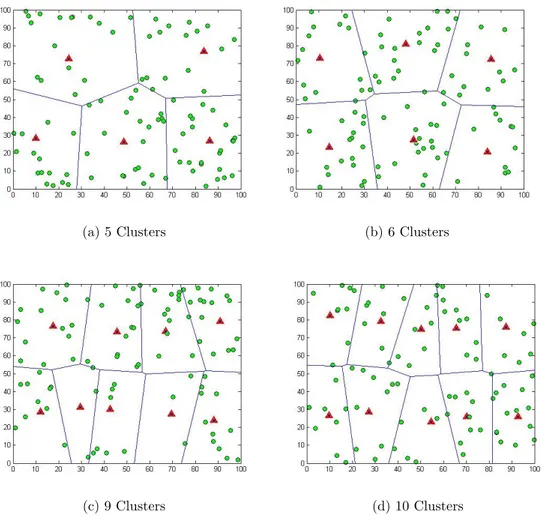
Since the clusters will remain fixed throughout the entire WSN lifetime, the initial cluster topologies are very important. Fig. 3.5 shows the cluster topologies based on intelligent CH selection mechanism of LEFCA for 5, 6, 9 and 10 clusters respectively. Depending on the desired number of clusters LEFCA selects the sensor nodes which are closest to the center of each cluster as the CHs. For example, if the desired number of clusters is 6, the network is split into 6 pieces and the nodes at the center (or closest to the center) of each piece become the CHs. The remaining nodes join to a CH which is nearest to their positions and the cluster topologies are formed.

3.1.2. Broadcast ADV Messages

Each node which has elected itself as a CH needs to notify the remaining nodes about the selection and later form the clusters for LEFCA algorithm. Once the nodes in LEFCA are elected to be CHs by BS, the CH nodes have to allow all the other nodes in the network that they have been elected for this

(51)

(a) 5 Clusters (b) 6 Clusters

(c) 9 Clusters (d) 10 Clusters

Figure 3.5: Cluster topologies for 5, 6, 9 and 10 clusters

task. To perform that, each CH broadcasts an ADV message which is shown in Fig. 3.6, using a non-persistent CSMA MAC protocol [68].

(52)

This advertisement message contains the ID of the CH and a header which recognizes that message as an advertisement message. To ensure that all nodes receive the advertisement message these messages are broadcasted into whole network by the CHs. Each regular node determines to which cluster it is related with by selecting the CH which needs the minimum communication energy, according to the received signal power of the ADV from each CH. Symmet-ric propagation channels for pure signal strength is assumed as the pure signal power attenuation of a message transmitted from a transmitting node to a re-ceiving node will be the identical with the attenuation of a message from the receiver to the transmitter. The traversing of the same path for both situations by electromagnetic wave provides symmetric propagation. This symmetric prop-agation provides nodes for hearing the CH advertisement with the largest signal strength thus, if they select the largest signal it means minimum transmitted energy is required for communication.

The rest of this subsection describes the CSMA approach used in proposed protocol.

Contrary to fixed-assignment access methods, with random-access meth-ods, the sources are not allocated to particular nodes. If a node holds data to transmit, it has to contend for accessing to the channel with another nodes for transmission. Therefore, collisions may happen when two nodes try to access to the channel simultaneously. This, in that case, will minimize overall throughput. Random-access methods aim to reduce collisions (and thus enhance throughput). The relative inefficiency of the existing medium access methods lies in the fact

(53)

that nodes do not take into account that other nodes what are making when they try to send data or control messages and this causes to large amount of collisions. Collisions can be prevented by using the idea that the nodes listen to the channel before sending data. This method, illustrated in Fig. 3.7, is called as listen-before-talk protocol, in other words CSMA [69].

Figure 3.7: Collision Mechanism in CSMA

CSMA is a kind of random access methods. In CSMA, when a node wants to send data, it pays attention to the channel to try to detect if another node is sending data at the same time. The usage of carrier-sense will minimize colli-sions, however it can not quarantee that collisions do not happen. For instance, there is a near-zero (not zero) that two nodes will detect the channel concur-rently, both make a decision that the channel is suitable for transmission, and both send data simultaneously, incuring a collision of both messages. The more presumedly collisions will happen because transmitter do not sense everything that the receiver can sense. In turn, the sender node supposes that the channel is idle for transmission, while the receiver node is making data reception from other node. This will give rise to a collision at the receiver, which will not be capable to receive data from any of transmitting node. This is named as the hidden terminal problem [70, 71]. The main problem is that collisions take place at the receiver but required to be sensed at the transmitter. In a wireless net-work by reason of the propagation lost of the radio signal, the transmitter do

(54)

not always get the identical message the receiver gets.

There are various di↵erent methods that are followed if the channel is occupied or free [72] for transmission. The node continues sensing until the channel is idle and then sends the data in 1-persistent CSMA. In here, 1 indicates the transmission method, that is to send with probability 1 immediately the channel is idle. After transmission, the sender node will wait for an ACK, if any ACK is reached to sender node in a particular amount of time, the sender node waits a random amount of time and then go back to listen to the channel. On the other hand, propagation delays have an important influence on 1-persistent CSMA. Yet this protocol can not exactly prevent collisions, and propagation delay a↵ects.

In non-persistent CSMA [73] - [75], a node does not listen to the channel all the time while it is busy. After detecting an occupied channel, the node waits a random amount of time before new detection. When the timer runs out, the node once more listens the channel. The node resets the timer if it is still busy, otherwise the node transmits the packet.

In 1-persistent CSMA [76], a node which has data to transmit begins send-ing its data instantly when the channel is free. However, the randomly deter-mined waiting times among channel detections prevent majority of the collisions which are occured because of simultaneous tranmissions of multiple nodes in non-persistent CSMA. Thus, non-persistent CSMA provides better throughput than 1-persistent CSMA at dense traffic.

(55)

Also with p-persistent CSMA, the channel is deemed to be divided into slots. The slot size is equal to the maximum propagation delay. The node listens the channel till it is idle, herein the node sends the data while the first convenient free slot with probability p. The throughput performance of the p-persistent CSMA can be placed between 1-persistent CSMA and non-persistent CSMA. In LEFCA, non-persistent CSMA is chosen because of its success in elimation of collisions and throuhgput performance which are analyzed and presented in detail in [77, 78].

In addition to collisions, packet drops can occur if the transmitter has to withdraw very long and the data are time-sensitive. There may be bu↵er overflow if the node has numerous packets to transmit and do not have accessing to the channel, eventuating in data losses.

Randomized approaches are simple to implement and they do not require network topology information. On the other hand, there are various disadvan-tages of these approaches. In wide shared-multimedia networks with frequent usage, collision can happen. Also, they are not energy-efficient because the radio electronics consume energy, carrier-sense and reception tasks are costly. With-out coordination between the nodes, random access methods need that the radio electronics are on further than is essential to transmit or receive data [79, 80].

(56)

3.1.3. Join Request Messages

After the members choose their clusters that they will join, these members must inform their associated CHs about their selection. Each node in a cluster sends a join-request message (Join-REQ) to the selected CH using again a non-persistent CSMA MAC protocol. This message contains the ID of the member node, the ID of the associated CH and a header. The structure of this message is given in Fig. 3.8. Note that, the length of these messages are fixed, and contrary to LEACH and LEACH based protocols, the transmission of these messages are realized only once in LEFCA because it uses fixed predefined clustering approach throughout all rounds instead of changing clusters for each round.

Figure 3.8: Join-REQ Message Structure of LEFCA

Fig. 3.9 shows an example for intelligent CH selection for LEFCA algo-rithm. For a 4 cluster topology, in each cluster, BS selects the CHs which are located centre of each cluster. For the 1st cluster, node 4 is selected as CH, for 2nd cluster, the CH is node 8, for cluster 3 the node 12 is elected as a CH and finally for 4rd cluster the CH node is node 16.

3.1.4. TDMA Schedule Messages

MAC Protocols try to solve the problem of multiple nodes sharing a com-mon channel. There are two di↵erent methods to divide the wireless channel between di↵erent nodes [81]:

(57)

Figure 3.9: Example for CH Selection in LEFCA

• Fixed-assignment channel access methods such as TDMA, FDMA, CDMA and SDMA

• Random access methods such as IEEE 802.11, CSMA, MACA and MACAW

Fixed-assignment channel access methods assign each node some amount of bandwidth, either dividing the spectrum in time (TDMA), frequency (FDMA), code (CDMA), or space (SDMA), thus, this allocation prevents collisions among data. Nevertheless, fixed-assignment schemes are not useful when some of the nodes are lacking in data transmission, as the bandwidth allocated to them will be wasted, while other nodes might be waiting to transmit their data.

Random access methods, do not allocate nodes fixed resources. They have contention-based nature such that nodes that have data to send have to attain bandwidth while diminishing collisions with the transmissions of another nodes.

(58)

In TDMA, time is divided into frames and a particular TS is assigned to each node within the frame to send its data [82]. Along this time-slot, another node cannot attain the channel, and collisions do not occur. The throughput in such a case is equivalent to the total data sent by every node.

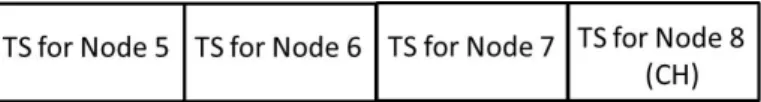
In LEFCA, once the clusters are formed, the CHs broadcast a TDMA schedule within its own cluster which includes allocated time slots (TSs) for each cluster member to transmit data. Also in each cluster, one extra TS is assigned for existing CH to transmit collected data from members to the BS. The length of the frame is determined based on the number of nodes (k) in the cluster (k+1 slots for each cluster, +1 for CH for each cluster). Fig. 3.10 shows an example of frame structure of a cluster in LEFCA.

Figure 3.10: Time slot assignment for cluster members in a LEFCA cluster

As an example the 4 cluster topology in Fig. 3.9 can be considered. For the second cluster, the assigned TSs can be determined for nodes 5,6,7 and the CH (node 8) as shown Fig. 3.11.

Figure 3.11: Example of Time slot assignment for cluster members in cluster 2 of Fig. 3.9

The TDMA schedule allocates specific time intervals for each of the clus-ter members to transmit their collected data to their CHs in LEFCA. TDMA

(59)

(a) The randomly deployed sensor nodes (b) The clusters and CHs after the set-up phase

Figure 3.12: Cluster Formation

schedule not only prevents the collisions among data messages but also enables the radio components of each regular node to put to sleep mode at all times except during their transmit time, thus providing energy savings.

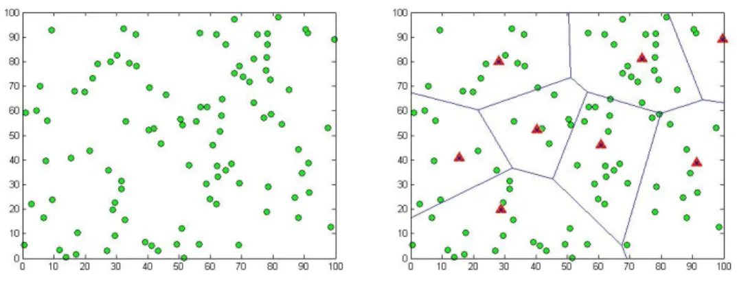
After the reception of the TDMA schedule by the cluster member nodes, the set-up phase is completed and data transmission with steady - state phase is ready to start. Fig. 3.12 (a) shows an example of randomly deployed sensor nodes in a WSN and Fig. 3.12 (b) shows an example illustration of the clusters formed after the LEFCA set-up phase.

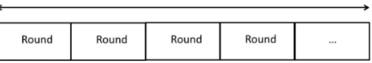
3.2. Steady-State Phase of LEFCA

The steady state phase of LEFCA is divided into repeating rounds as shown in Fig. 3.13. Each round consists of data transmission phase and CH change decisision phase.

(60)

Figure 3.13: The Steady State Phase of LEFCA

The main objective of the steady-state phase is to transmit the collected data to the base station through the CHs and to determine whether a CH change needs to be made. Fig. 3.14 shows a typical round for the LEFCA algorithm with its two sub phases: data transmission and CH change decision.

Figure 3.14: The LEFCA Round. Data transfers and changing of CHs if needed occur during the steady-state phase.

3.2.1. Data Transmission Phase

This phase is divided into slots allocated for each of the cluster members, where the member nodes transmit their data to the CH. The duration for each slot is fixed, thus the time to transmit data hinges on the number of member nodes in the cluster. When the data collection from the cluster members is complete, the CH transmits collected data to the base station.

(61)

Spread spectrum communications and CDMA [83] - [91] are significant technologies which provide various nodes to transmit concurrently utilizing the bandwidth by spreading their data by use of a unique spreading code.

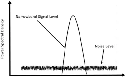
Figure 3.15 shows a narrow band signal in the frequency spectrum. These narrow band signals can be readily jammed by any other signal in the same band. In the same way, the signal may be intercepted because the frequency band is fixed and narrow.

Figure 3.15: Narrow band signal.

The idea of spread spectrum is to use more bandwidth than the original message while sustaining equal signal power. A spread spectrum signal does not have a clearly perceptible peak in the spectrum. This makes the signal harder to separate from noise and hence harder to jam or intercept [92].

(62)

system [93]:

DS-SS introduces rapid phase transition to the data doing it bigger in bandwidth. As the period T of a signal shortens in time, the bandwidth B of the signal enlarges: R = 1/T = 2B. The rapid phase transition signal has a greater bandwidth given that the rate is bigger and acts like as noise in this case their spectrums become similar for bandwidth in scope. Actually, the power density amplitude of the spread spectrum output signal is similar to the noise floor. The signal is hidden under the noise.

To retrieve the signal, the certain same wide bandwidth signal is required. This is like a key, the demodulator which includes a key can be used to obtain signal back. This key is indeed a PN sequence. These sequences are generated by m-sequences. DS-SS codes will all be trimmed as PN sequences since are similar to random sequences of bits with a flat noise-like spectrum. To obtain noise-like spectrum, the sequence must be long enough (according to the message signal). This is the relation between chip rate which is shown as Rc = 1/Tc and message rate that is Rb= 1/Tb. Thus, spreading factor becomes: N = Tb/Tc. In practical systems, N is an integer which corresponds to the number of chips per information bit. In here, the transmission power is spread over a bandwidth N times wider than the information symbol rate, the spectral length of the signal is N times lower than it would be in nonspread transmission. The amplitudes of the chips are coded in a periodic random-appearing pattern referred to as the spreading code. Optimally, the spreading code is designed so that the chip amplitudes are statiscally independent of each other. As the chip sequence is

(63)

coded to appear random. If the period of the spreading code is one period of the spreading signal can be denoted by

f (t) = N X

i=1

bip(t iTc) (3.1)

where N is the number of chips per bit, p(t) is the chip pulse shape, and bi are the values of the PN chips. Thus, spreading signal becomes:

f (t) =X k

f (t kTb) (3.2)

The transmitted baseband signal is then given by

f (t) =X k

anf (t nTb) (3.3)

where an is the information digit. The autocorrelation function of the trans-mitted signal and the duplicate of the periodic PN spreading signal is given by Rxs(⌧ ) = X n anRf f(⌧ nTb) (3.4) where Rxs(⌧ ) = Z 1 1 f (t)f (t + ⌧ ) (3.5)

(64)

In here, if the transmitted bit symbol is 1, stated by a positive voltage level, the peaks of the correlation function will become positive. If the transmitted bit symbol is 0, represented by a negative voltage level, the related peak at the receiver is negative. For this reason, the information bits symbolized by a fixed voltage value with duration Tb at the input to the transmitter. These information bits are expressed by narrow pulses with width twice the chip du-ration after cross-correlation at the receiver. The genedu-ration of the peak of the autocorrelation function provides to design a simple receiver.

The spread-spectrum scheme is named as a two-layer modulation tech-nique. In the standart analog modulation techniques (i.e. AM, DSB, SSB), the message signal is multiplied by a sinusoidal carrier. On the other hand, the information signal is multiplied by a spreading signal in the spread-spectrum modulation systems. The spread-spectrum demodulator correlates the received signal with a transcribe of the random carrier. However, the standart demodu-lator correlates the received signal with a duplicate of the transmitted sinusoid.

The CDMA technology is built on spread-spectrum transmission and re-ception. All nodes use the same carrier frequency and may transmit simultane-ously in CDMA system. Each unique spreading code is approximately orthogo-nal to all other codewords.

The number of synchronous transmissions in a CDMA method is [95]:

N = ⌘bcd Bw RbE_I_ob