YAŞAR UNIVERSITY
GRADUATE SCHOOL OF NATURAL AND APPLIED SCIENCES
MASTER THESIS
COMPARISON OF LINEAR ORDINARY
DIFFERENTIAL EQUATIONS SOLUTION METHODS
AND THEIR APPLICATIONS
Cansu AYVAZ
Thesis Advisor: Assist. Prof. Dr. Refet POLAT
Department of Mathematics
Presentation Date: 28.01.2016
Bornova-İZMİR 2016
ii
iii ABSTRACT
COMPARISON OF LINEAR ORDINARY DIFFERENTIAL EQUATIONS SOLUTION METHODS
AND THEIR APPLICATIONS AYVAZ, Cansu
M.Sc in Department of Mathematics Supervisor: Assist. Prof. Dr. Refet POLAT
January 2016, 114 pages
In the first section of this thesis, an introduction about the development of differential equation and definitions of the subject are given. In the second chapter, methods that are necessary for reaching the solution of differential equations are given. The method in applied mathematics can be an effective procedure to obtain analytical and approximate solutions for different types of operator. In the third chapter, inspected articles about linear ordinary differential equation, and their synthesis are given. In the fourth chapter, various applications areas of linear ordinary differential equations like economics, biology, mechanics are given. Finally in fifth chapter a conclusion is given.
Keywords: Linear Ordinary Differential Equation, Economic problems, Mechanic Problems.
iv ÖZET
LİNEER ADİ DİFERANSİYEL DENKLEMLER ÇÖZÜM YÖNTEMLERİNİN KARŞILAŞTIRILMASI
VE UYGULAMALARI Cansu AYVAZ
Yüksek Lisans, Matematik Bölümü Tez Danışmanı: Yrd. Doç. Dr. Refet POLAT
Ocak 2016, 114 sayfa
Bu tezin ilk bölümünde diferansiyel denklemlerin oluşumundan bahsedilmiş ve ilgili tanımlar verilmiştir. İkinci bölümünde çözüme ulaşmak için gerekli metotlar vardır. Uygulamalı matematikte yöntem, farklı tipte operatörler için analitik ve yaklaşık çözümler elde etmede etkili bir prosedürdür. Üçüncü bölümde lineer adi diferansiyel denklemler ile ilgili incelenen makaleler, ve sentezi verilmiştir. Dördüncü bölümde ise lineer adi diferansiyel denklemlerin ekonomi, biyoloji, mekanik gibi çeşitli alanlarda uygulamaları verilmiştir. Son olarak beşinci bölümde sonuç verilmiştir.
Anahtar sözcükler: Lineer Adi Diferansiyel Denklem, Ekonomi Problemleri,Mekanik Problemler
v
ACKNOWLEDGEMENTS
I would like to thank to my supervisor Assist. Prof. Dr. Refet POLAT for his support and help on my thesis.
Cansu AYVAZ İzmir, 2016
vi
TEXT OF OATH
I declare and honestly confirm that my study, titled “COMPARISON OF LINEAR ORDINARY DIFFERENTIAL EQUATIONS SOLUTION METHODS AND THEIR APPLICATIONS” and presented as a Master’s Thesis, has been written without applying to any assistance inconsistent with scientific ethics and traditions, that all sources from which I have benefited are listed in the bibliography, and that I have benefited from these sources by means of making references.
vii TABLE OF CONTENTS Page ABSTRACT iii ÖZET iv ACKNOWLEDGEMENTS v TEXT OF OATH vi
TABLE OF CONTENTS vii
INDEX OF FIGURES xi
INDEX OF TABLES xii
1 INTRODUCTION 1
1.1 Calculus Review 2
1.1.1 Derivatives 2
1.1.2 Anti-derivatives and Indefinite Integral 6
1.1.3 Definite Integrals 9
1.2 Introduction to Differential Equations 12
1.2.1 Definitions 12
1.2.2 Classifications of Differential Equations 13
viii
1.2.4 Modeling a Differential Equation 17
2 REVIEW OF THE LITERATURE 19
2.1 First Order Linear Differential Equations 19
2.1.1 Homogeneous and Nonhomogeneous Equations 19
2.1.2 Solution of Homogenous Equation 20
2.1.3 Solution of The Nonhomogeneous Equation 21
2.1.4 Exact Differential Equations and Integrating Factors 24
2.1.4.1 Exact Differential Equations 24
2.1.4.2 Integrating Factors 26
2.2 Higher Order Linear Differential Equations 26
2.2.1 Introduction 27
2.2.2 Linear Independency and Wronskian Functions 28
2.2.3 Homogeneous Equations Theory 32
2.2.4 Constant Coefficient Homogenous Differential Equations 32
2.2.4.1 The Characteristic Equation 32
2.2.4.2 Multiple Zeros of The Characteristic Equation 36
2.2.5 Nonhomogeneous Equations Theory 40
ix
2.2.5.2 The Method of Variation of The Constants 43
2.2.6 Euler Equations 48
2.3 Linear Differential Equation Systems 52
2.3.1 Elimination Method 56
2.3.2 Eigenvalue Method 58
2.3.2.1 Distinct Real Eigenvalues 61
2.3.2.2 Complex Eigenvalues 64
2.3.3 Comparison of Methods 67
3 INSPECTED ARTICLES 69
3.1 Statistical Modeling of Breast Cancer 69
3.2 Analysis of Economic Growth Differential Equation 77 3.3 Numerical Solution of Vintage Capital Growth Models 83
3.4 Synthesis 86
4 APPLICATIONS OF LINEAR DIFFERENTIAL EQUATIONS 88
4.1 Economic Problems 88
4.2 Biologic Problems 92
4.3 Mechanic Problems 94
x 4.3.2 Spring Problems 101 4.4 Electric Circuits 105 5 CONCLUSION 111 REFERENCES 112 CURRICULUM VITEA 114
xi
INDEX OF FIGURES
Figure 1.1 The slope of the tangent line at from Weir (2010) 3
Figure 1.2 The curves from Weir (2010) 7
Figure 2.1 Direction field of the diff. eq. from Collatz (1986) 23 Figure 2.2 Direction field of the diff. eq. from Collatz (1986) 23 Figure 2.3 Direction field of the diff. eq. from Collatz (1986) 23
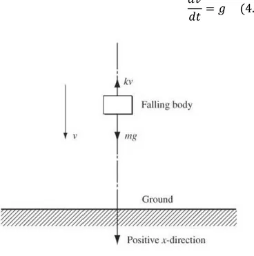
Figure 2.4 Direction field and solution curves for the linear system 64 Figure 3.1 Average Tumor Size x Age tabulation from Tsokos and Xu (2011) 74 Figure 3.2 Tumor Size IROC x Age tabulation from Tsokos and Xu (2011) 75 Figure 4.1 Falling body with air resistance from Bronson and Costa (2006) 95
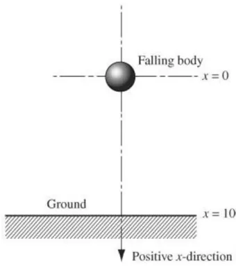
Figure 4.2 Falling Body from Bronson and Costa (2006) 96
Figure 4.3 Rising body from Bronson and Costa (2006) 98
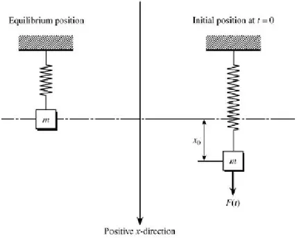
Figure 4.4 Spring from Bronson and Costa (2006) 101
Figure 4.5 RL Circuit from Bronson and Costa (2006) 107
Figure 4.6 RC Circuit from Bronson and Costa (2006) 107
xii
INDEX OF TABLES
Table 1.1 Other notations for the derivative (Weir 2010) 4
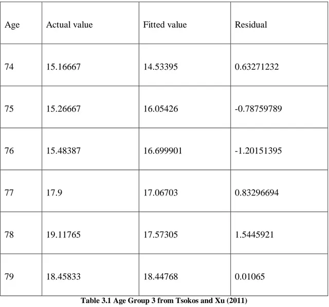
Table 3.1 Age Group 3 from Tsokos and Xu (2011) 73
Table 3.2 Residuals of Age Group 3 from Tsokos and Xu (2011) 73
Table 3.3 Age Group 3 IROC from Tsokos and Xu (2011) 76
1 1 INTRODUCTION
Mathematics as a science commenced when first someone, probably a Greek, proved propositions about any things or about some things, without specification of definite particular things. These propositions were first enunciated by the Greeks for geometry; and, accordingly, geometry was the great Greek mathematical science. After the rise of geometry centuries passed away before algebra made a really effective start, despite some faint anticipations by the later Greek mathematicians (Whitehead, 1958).
The ideas of any and of some are introduced into algebra by the use of letters, instead of the definite numbers of arithmetic. Thus, instead of saying that 2+3 = 3+ 2, in algebra we generalize and say that, if x and y stand for any two numbers, then x+y= y+x. Again, in the place of saying that 3 > 2, we generalize and say that if x be any number there exists some number (or numbers) y such that y > x. We may remark in passing that this latter assumption - for when put in its strict ultimate form it is an assumption - is of vital importance, both to philosophy and to mathematics; for by it the notion of infinity is introduced. Perhaps it required the introduction of the Arabic numerals, by which the use of letters as standing for definite numbers has been completely discarded in mathematics, in order to suggest to mathematicians the technical convenience of the use of letters for the ideas of any number and some number. The Romans would have stated the number of the year in which this is written in the form MDCCCCX, whereas we write it 1910, thus leaving the letters for the other usage. But this is merely a speculation. After the rise of algebra the differential calculus was invented by Newton and Leibniz, and then a pause in the progress of the philosophy of mathematical thought occurred so far as these notions are concerned; and it was not till within the last few years that it has been realized how fundamental any and some are to the very nature of mathematics, with the result of opening out still further subjects for mathematical exploration (Whitehead, 1958).
In this project, differential calculus is going to be examined. The word Calculus comes from Latin meaning "small stone". Because it is understanding something by looking at small pieces. Differential Calculus cuts something into small pieces to find how it changes. For example, differential calculus helps to know some distance over
2
some time. This is differential equation. In another saying, differential equations are inescapable to come up with a solution with time dependent scientific problems.
The subject of differential equations constitutes a large and very important branch of modern mathematics. In physics, engineering, chemistry, economics, and other sciences mathematical models are built that involve rates at which things happen. These models are equations and the rates are derivatives. Equations containing derivatives are called differential equations.(Ross,2004)
A review of calculus is given below. 1.1 Calculus Review
In this section, the slope and tangent to a curve at a point, and the derivative of a function at a point are defined. Later in the chapter, the derivative as the instantaneous rate of change of a function is interpreted, and this interpretation applied to the study of certain types of motion. By reviewing Weir (2010).
1.1.1 Derivatives
To find a tangent to an arbitrary curve at a point , the slope of the secant through and a nearby point is calculated. Then the limit of the slope as (Fig. 1.1) is investigated. If the limit exists, it is called as the slope of the curve at and defined as the tangent at to be the line through having this slope (Weir,2010).
3
Figure 1.1 The slope of the tangent line at from Weir (2010)
Definition 1.1: The slope of the curve at the point is the number
provided the limit e ists .
The tangent line to the curve at P is the line through with this slope (Weir,2010).
The expression
is called the difference quotient of at with increment . If the difference quotient has a limit as approaches zero, that limit is given a special name and notation. Definition 1.2: The derivative of a function at a point , denoted , is
4 provided this limit exists (Weir,2010).
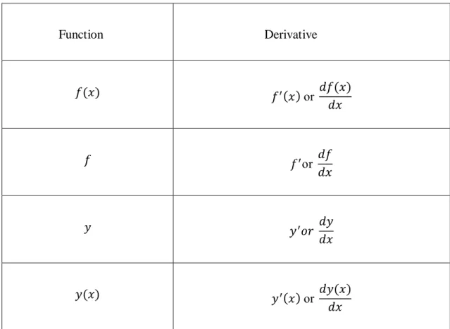
Other notations for the derivative of a function is given Table below.
Function Derivative or or or
Table 1.1 Other notations for the derivative from Weir (2010)
A function is differentiable on an open interval (finite or infinite) if it has a derivative at each point of the interval. It is differentiable on a closed interval if it is differentiable on the interior and if the limits
ight hand derivative at
Left hand derivative at
exist at the endpoints (Weir,2010).
Right-hand and left-hand derivatives may be defined at any point of a function's domain. According to Weir (2010) a function has a derivative at a point if and only if
5
it has left-hand and right-hand derivatives there, and these one-sided derivatives are equal.
If is a differentiable function, then its derivative is also a function. If is also differentiable, then we can differentiate to get a new function of denoted by so The function is called the second derivative of
because it is the derivative of the first derivative (Weir,2010).
For higher order derivatives the notations are
or
eir,2010 .
To get a better understanding of subject, at first, derivatives of the most commonly used elementary functions are given below and differentiation rules are given after;
Rules of Differentiation are listed below, If has the constant value then
6
If is a positive integer, then
If is a differentiable function of and is a constant, then
If and are differentiable functions of then their sum is differentiable at every point where and are both differentiable. At such points,
If and are differentiable at then so is their product , and
If and are differentiable at and if then the quotient is differentiable at , and
eir,2010
1.1.2 Anti-derivatives and Indefinite Integral
It have been studied that how to find the derivative of a function. However, many problems require that we recover a function from its known derivative (from its known rate of change). For instance, we may know the velocity function of an object
7
falling from an initial height and need to know its height at any time. More generally, we want to find a function from its derivative . If such a function exists, it is called an antiderivative of . We will see in the next chapter that antiderivatives are the link connecting the two major elements of calculus: derivatives and definite integrals (Weir,2010).
Definition 1.3: A function is an antiderivative of on an interval if for all in (Weir,2010).
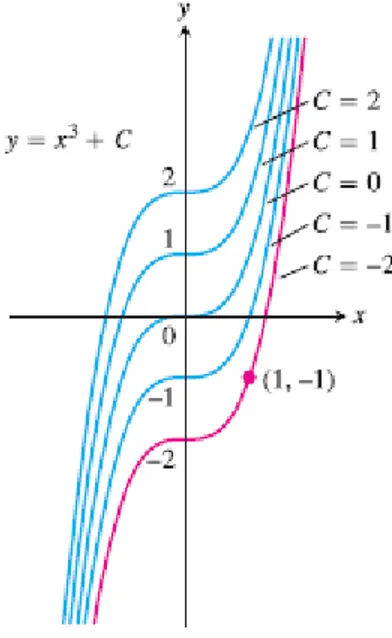
Thus the most general antiderivative of on is a family of functions whose graphs are vertical translations of one another. A particular antiderivative from this family can be selected by assigning a specific value to C. Here is an example showing how such an assignment might be made;
Example 1.1: Find an antiderivative of that satisfies
Figure 1.2 The curves from Weir (2010)
Solution: Since the derivative of is , the general antiderivative
8
gives all the antiderivatives of . The condition determines a specific value for . Substituting into gives
.
Since , solving for gives . So
is the antiderivative satisfying . Notice that this assignment for selects the particular curve from the family of curves that passes through the point
in the plane (Figure 1.2) (Weir,2010).
A special symbol is used to denote the collection of all antiderivatives of a function .
Definition 1.4: The collection of all antiderivatives of is called the indefinite integral of with respect to , and is denoted by
The symbol is an integral sign. The function is the integrand of the integral, and is the variable of integration (Weir, 2010).
This notation is related to the main application of antiderivatives. According to Weir, (2010) antiderivatives play a key role in computing limits of certain infinite sums, an unexpected and wonderfully useful role, called the Fundamental Theorem of Calculus. It connects integration and differentiation, enabling us to compute integrals using an antiderivative of the integrand function rather than by taking limits of Riemann sums.
9 1.1.3 Definite Integrals
Definition 1.5: Let be a function defined on a closed interval We say that a number is the definite integral of over and that is the limit of the Riemann sums if the following condition is satisfied:
Given any number there is a corresponding number such that for every partition of with and any choice of in we have
The definition involves a limiting process in which the norm of the partition goes to zero. In the cases where the subintervals all have equal width
, we can form each Riemann sum as
where is chosen in the subinterval . If the limit of these Riemann sums as exists and is equal to , then is the definite integral of over , so
Leibniz introduced a notation for the definite integral that captures its construction as a limit of Riemann sums. He envisioned the finite sums
becoming an infinite sum of function values multiplied by
10
the integral symbol , whose origin is in the letter "S." The function values are replaced by a continuous selection of function values The subinterval widths become the differential . It is as if we are summing all products of the form as goes from to . While this notation captures the process of constructing an integral, it is Riemann's definition that gives a precise meaning to the definite integral (Weir,2010).
The symbol for the number in the definition of the definite integral is
After indefinite and definite integrals now Fundamental Theorem of Calculus and rules for integration can be given.
The Fundamental Theorem of Calculus (FTC):
Part 1 If is continuous on then is continuous on and differentiable on and its derivative is
eir,2010
Part 2 If is continuous at every point of and is any antiderivative of on , then
Integration Rules;
Zero:
11 Order of Integration Constant Multiples:
Sums and Differences:
Additivity:
Max-Min Inequality: If max and min are the maximum and minimum values of on then
12 Domination:
(Weir,2010). 1.2 Introduction to Differential Equations
The study of differential equations has attracted the attention of many of the world’s greatest mathematicians during the past three centuries. Nevertheless, it remains a dynamic field of inquiry today, with many interesting open questions. Now detailed informations about differential equations will be given.
1.2.1 Definitions
Definition 1.6: An equation involving derivatives of one or more dependent variables with respect to one or more independent variables is called a differential equat ion (Ross, 2004).
Some examples of differential equations listed below.
13
From the brief list of differential equations examples above it is clear that the various variables and derivatives involved in a differential equation can occur in a variety of ways. Clearly some kind of classification must be made. Therefore, differential equations are classified according to the specified properties which are given below.
1.2.2 Classifications of Differential Equations
From the early days of the calculus subject of differential equations has been an area of great theoretical research and practical applications, and it continues to be so in our day. This much stated several questions naturally arise. Just what is a differential equation and what does it signify? Where and how do differential equations originate and of what use are they? Confronted with a differential equation, what does one do with it, how does one do it, and what are the results of such activity? These questions indicate three major aspects of the subject: theory, method, and application (Ross, 2004).
To begin with, differential equations are classified according to whether there is one or more than one independent variable involved.
Definition 1.7: A differential equation involving ordinary derivatives of one or more dependent variables with respect to a single independent variable is called an ordinary differential equation (Ross, 2004).
As example, Equations (1.1) and (1.2) are ordinary differential equations. In Equation (1.1) the variable is the single independent variable, and is a dependent variable. In Equation (1.2) the independent variable is , whereas is dependent.
Definition 1.8: A differential equation involving partial derivatives of one or more dependent variables with respect to more than one independent variable is called a partial differential equation (Ross, 2004).
As example, Equations (1.3) and (1.4) are partial differential equations. In Equation (1.3) the variable and are independent variables and is a dependent variable. In Equation (1.4) there are three independent variables: and ; in this equation is dependent.
14
Differential equations further classified, both ordinary and partial, according to the order of the highest derivative appearing in the equation. For this purpose following definition is given (Ross,2004).
Definition 1.9: The order of the highest ordered derivative involved in a differential equation is called the order of the differential equation (Ross, 2004).
As example, the ordinary differential equation (1.1) is of the second order, since the highest derivative involved is a second derivative. Equation (1.2) is an ordinary differential equation of the fourth order. The partial differential equations (1.3) and (1.4) are of the first and second orders, respectively.
Proceeding with this study of ordinary differential equations, the important concept of linearity applied to such equations is going to be introduced now. This concept will enable these equations to classify still further.
Definition 1.10: A linear ordinary differential equation of order , in the dependent variable and the independent variable , is an equation that is in, or can be expressed in, the form
where is not identically zero.
Observe (1) that the dependent variable and its various derivatives occur to the first degree only, (2) that no products of and/or any of its derivatives are present, and (3) that no transcendental functions of and/or its derivatives occur (Ross,2004).
Several examples of linear differential equations are given below.
The following ordinary differential equations are both linear. In each case is the dependent variable. Observe that and its various derivatives occur to the first degree only and that no products of and/or any of its derivatives are present.
15 Definition 1.11: A nonlinear ordinary differential equation is an ordinary differential equation that is not linear (Ross, 2004).
Some examples of nonlinear ordinary differential are given below.
Equation (1.7) is nonlinear because the dependent variable appears to the second degree in the term . Equation (1.8) owes its nonlinearity to the presence of the term , which involves the third power of the first derivative. Finally, Equation (1.9) is nonlinear because of the term , which involves the product of the dependent variable and its first derivative.
Linear ordinary differential equations are further classified according to the nature of the coefficients of the dependent variables and their derivatives (Ross,2004).
Definition 1.12: A linear differential equation has constant coefficients if the coefficients of are all constants (Ross, 2004).
Definition 1.13: A linear differential equation has variable coefficients if the are multiplied by any variable (Ross, 2004).
16
For example, Equation (1.5) is said to be linear with constant coefficients, while Equation (1.6) is linear with variable coefficients.
1.2.3 Initial Value Problems
A problem in which we are looking for the unknown function of a differential equation where the values of the unknown function and its derivatives at some point are known is called an initial value problem.
Antiderivatives play several important roles in mathematics and its applications. Methods and techniques for finding them are a major part of calculus. Finding an antiderivative for a function is the same problem as finding a function that satisfies the equation
This is called a differential equation, since it is an equation involving an unknown function that is being differentiated. To solve it, we need a function that satisfies the equation. This function is found by taking the antiderivative of . We fix the arbitrary constant arising in the anti-differentiation process by specifying an initial condition
This condition means the function has the value when . The combination of a differential equation and initial conditions is called an initial value problem. Such problems play important roles in all branches of science (Weir,2010). A simple example is going to be considered for this chapter.
Example 1.2 Find a solution of the differential equation
Such that at this solution has the value .
17
Explanation and Solution: First let us be certain that we thoroughly understand this problem. We seek a real function of which fulfills the two following requirements:
First, The Function must satisfy the differential equation (1). That is, the function must be such that for all real in a real interval .
Second, The function must have the value 4 at . That is, the function must be such that .
Equation (1) has a solution which is written as
where is an arbitrary constant, and that each of these solutions satisfies the first requirement that is mentioned above. let us now attempt to determine the constant so that (2) satisfies the second requirement, that is, at Substituting into (2), we obtain and hence . Now substituting the value thus determined back into (2), we obtain
which is indeed a solution of the differential equation (1), which has the value at In other words, the function defined by
satisfies both of the requirement set forth in the problem (Ross,2004). 1.2.4 Modeling a Differential Equation
Since many of the fundamental laws of the physical and social sciences involve rates of change, it should not be surprising that such laws are modeled by differential equations (Anton et al., 2012). In this section the general idea of modeling with differential equations is going to be discussed, and in the third and fourth chapter, some important methods that can be applied to population growth, medicine, mechanics, electrics and ecology are going to be investigated.
18
Differential equations are of interest to nonmathematicians primarily because of the possibility of using them to investigate a wide variety of problems in the physical, biological, and social sciences. One reason for this is that mathematical models and their solutions lead to equations relating the variables and parameters in the problem. These equations often enable you to make predictions about how the natural process will behave in various circumstances. (Boyce and Diprima, 2001).
Recall that a differential equation is an equation involving one or more derivatives of an unknown function.
Examples of modeling and applications of differential equations are given in third and fourth chapters more detailed. Now a review of literature is given for solution methods that are being used in differential equations.
19 2 REVIEW OF THE LITERATURE
There are many real life problems that can be modeled by means of differential equations. Especially ordinary differential equations have been used in physical sciences about 17th-18th centuries. Although there are some methods to find the exact solutions of them, it is a well-known fact that any differential equation does not have general solution. For that reason approximate or numerical solutions of differential equation have been studied by researchers for a long time (Kara,2015).
2.1 First Order Linear Differential Equations
There are many physical problems that involve a number of separate elements linked together in some manner. For example, electrical networks have this character, as do some problems in mechanics or in other fields. In these and similar cases the corresponding mathematical problem consists of a system of two or more differential equations, which can always be written as first order equations. In this chapter systems of first order linear equations are given (Boyce and Diprima,2001).
2.1.1 Homogeneous and Nonhomogeneous Equations
Another integrable type of differential equation is the so-called linear differential equation
and are given functions, perhaps continuous; for example, is such a linear equation.
If still has a function as a factor, the whole equation is to be divided by this function, provided that .
If the right-hand side vanishes identically, the equation is said to be homogeneous. Thus is the homogeneous equation corresponding to the above example.
20
But if the right-hand side does not vanish identically, i.e., if , then the differential equation is said to be nonhomogeneous. In such an equation is called the `perturbing function' or the `perturbing term'.
The nomenclature homogeneous and nonhomogeneous is analogous to that used for linear systems of algebraic equations. Homogeneous linear systems of equations in algebra always have the so-called `trivial' solution (all the unknowns are zero), but the `non-trivial solutions' are of special interest.
The homogeneous linear differential equation
also has a trivial solution, namely, ; its graph is the -axis. But there are 'non-trivial solutions' as well, and it is these in which we are much more interested (Collatz,1986).
2.1.2 Solution of Homogenous Equation Separation of the variables in (2.2) gives
Let denote an antiderivative of the integral on the right; then
Hence
For the sake of clarity the letter has been used as the variable of integration to distinguish it from the upper limit of the integral. It does not matter what lower
21
limit is chosen; often is convenient (of course, must lie in the domain of the function ) (Collatz,1986).
Example 2.1
The solution is
or, taking as the lower limit and writing
For or we obtain the trivial solution (Collatz,1986).
2.1.3 Solution of The Nonhomogeneous Equation
The homogeneous equation has the general solution with as an arbitrary constant. We wish to try to account for the `distortion' of the solution by the `perturbing term' by putting , i.e., we transform the differential equation (2.1) into a new one for the function , hoping that the new equation will be simpler. Thus in place of the constant a function , which is to be determined, appears; the method is therefore known as the method of variation of the constants (Lagrange). From
it follows that
22
Substitution into the differential equation (2.1) gives
By integrating we obtain immediately
So the general solution of the nonhomogeneous linear differential equation (2.1) is
The method of variation of the constants can also be applied to linear differential equations of higher order (Collatz,1986). An example about nonhomogeneous equations is given below.
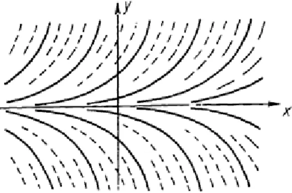
Example 2.2 To illustrate the effect of the ‘perturbing function’ we compare the direction fields of the differential equations
homogeneous linear
23
Figure 2.1 Direction field of the diff. eq. from Collatz (1986)
Figure 2.2 Direction field of the diff. eq. from Collatz (1986)
24 Their general solutions are:
igure 2.1 igure 2.2 igure 2.
(Collatz, 1986). 2.1.4 Exact Differential Equations and Integrating Factors
For first order equations there are a number of integration methods that are applicable to various classes of problems. The most important of these are linear equations and separable equations, which is discussed previously. Here, a class of equations known as exact equations is considered for which there is also a well-defined method of solution. Keep in mind, however, that those first order equations that can be solved by elementary integration methods are rather special; most first order equations cannot be solved in this way (Boyce and Diprima, 2001).
2.1.4.1 Exact Differential Equations
Let a differential equation be written in the form
This is called an exact differential equation if
and then constant is the general solution in implicit form. Now it is well known that the mixed second derivatives of a function are identical with one another provided they are continuous:
25
hence we obtain a simple necessary condition for a differential equation to be exact, viz.,
However, cases where a differential equation satisfies this condition immediately rarely occur (Collatz,1986). An example is given below for exact differential equations.
Example 2.3 Solve the differential equation
Solution The equation is neither linear nor separable, so the methods suitable for those types of equations are not applicable here. However, observe that the function has the property that
Therefore the differential equation can be written as
Assuming that is a function of and calling upon the chain rule, we can write Equation (3) in the equivalent from
Therefore
26
where is an arbitrary constant, is an equation that defines solution of Equation (1) implicitly (Boyce and Diprima, 2001).
2.1.4.2 Integrating Factors
Sometimes, however, a differential equation can easily be changed into an exact differential equation by multiplying it throughout by a suitable, so-called integrating factor . We therefore require of that for
the condition
shall be satisfied, or, differentiating out,
At first sight it seems as if the difficulties have been increased, because now, instead of an ordinary differential equation, we have to solve a partial differential equation for the function . But sometimes a particular solution of this partial differential equation can be guessed, and any one solution (which must, of course, not vanish identically) is all that is needed (Collatz,1986).
2.2 Higher Order Linear Differential Equations
Linear equations of higher order are of crucial importance in the study of differential equations for two main reasons. The first is that linear equations have a rich theoretical structure that underlies a number of systematic methods of solution. Further, a substantial portion of this structure and these methods are understandable at a fairly elementary mathematical level. Another reason to study second and higher order linear equations is that they are vital to any serious investigation of the classical areas of mathematical physics. One cannot go very far in the development of fluid
27
mechanics, heat conduction, wave motion, or electromagnetic phenomena without finding it necessary to solve second order linear differential equations. For examples see Chapter 4. (Boyce and Diprima,2001)
2.2.1 Introduction
A very important type of differential equation of higher order is the linear differential equation. It has, compared to (2.1), the general form
We also write the entire left-hand side briefly and symbolically as , thus
In this expression the zeroth derivative means the function itself. The and are given continuous functions of in an interval . As in Chapter 2.1.1, we call the differential equation homogeneous if , otherwise nonhomogeneous. If in , then we can divide (2.3) by , and we obtain an equation with continuous coefficients, for which the theorem in is applicable; according to this theorem, if the initial conditions for , where must, of course, be in , are prescribed, then the solution of the differential equation is uniquely determined. If nothing to the contrary is stated, we shall in the following assume (Collatz,1986).
is a linear homogeneous differential expression, which has these properties: if are two n-times continuously differentiable functions and if is an arbitrary constant, then
28 In particular,
2.2.2 Linear Independency and Wronskian Functions
There is a criterion for linear independence of solutions of an nth -order homogeneous differential equation.
First of all, let be any given functions which are times continuously differentiable in an interval (Collatz,1986). Now suppose that these functions are linearly dependent in ; then there are constants , not all zero, such that the combination
vanishes identically in ; but then the same is true for the derivatives
This is a system of n linear homogeneous equations for the quantities . According to Collatz (1986) it has a non-trivial solution, and so the determinant of the system of equations must have the value zero (at every point of the interval); this determinant is called the Wronskian determinant, or simply the Wronskian:
29
Now the identical vanishing of the Wronskian is indeed a necessary, but by no means a sufficient, condition for linear dependence of the functions . For example the functions defined and continuously differentiable in the interval are linearly independent, but nevertheless their Wronskian vanishes identically:
If, however, it is additionally assumed that the are solutions of a homogeneous differential equation of order , then the vanishing of the Wronskian is a criterion for linear dependence. This will now be made more precise.
Let be solutions in an interval of the homogeneous differential equation
where, as before, the are given continuous functions in with The Wronskian of the functions , formed as in (2.6), then satisfies a simple differential equation. To set up this equation we form the derivative of . A determinant is differentiated by differentiating each row in turn, keeping the other rows unchanged, and adding the determinants so formed. Thus
The first determinants on the right vanish, because in each there are two identical rows; so only the last determinant remains. In it we multiply the last row by , so that the value of the determinant is likewise multiplied by ; then we multiply the first row by , the second row by , and so on, and finally the (n-1)th row by , and add the products to the nth row; the value of
30
the determinant is unchanged by so doing. The terms in the last row are thus replaced by
But from the differential equation (2.7) this is precisely equal to , and so we can take the factor , outside the determinant and thus obtain the original Wronskian; so
This linear differential equation of the first order for has the solution
Here is an arbitrarily chosen point in . If, therefore, (resp. ) at a point , then (resp. ) throughout the entire interval , since the exponential factor is always ; the Wronskian of the solutions either vanishes identically or vanishes nowhere in the interval . It was proved earlier that if the are linearly dependent in then vanishes identically. But the converse also holds: if vanishes at a point in (and therefore identically), then the are linearly dependent in . Since , the system of equations (2.4), (2.5) written for the point has a non-trivial solution ,and the function
formed using these constants is a solution of the homogeneous differential equation, with the initial values at the point
31
But this initial-value problem has the solution , and since the initial-value problem has a unique solution, we must have in , i.e., the solutions are linearly dependent. So the following theorem holds (Collatz,1986).
Theorem 2.1 solutions of a homogeneous linear nth-order differential equation (2.7) with continuous coefficients and in an interval form a fundamental system, i.e., are linearly independent, if and only if their Wronskian (2.6) is different from zero at an arbitrarily chosen point of the interval (Collatz,1986).
And an example of this chapter is below.
Example 2.4 It can be shown immediately by substitution that (for ) and
satisfy the differential equation
their Wronskian at, say, the point , is non-zero:
so the general solution of (1) reads
a normalized fundamental system for the point is formed by the functions
is the solution of the initial-value problem for (1) with the initial conditions (Collatz,1986).
32
2.2.3 Homogeneous Equations Theory
Let us look the solution of differential equation. Assuming that general solution of , and , we can figure Çengel,201 . According to this, we can write the principle of superposition below.
“If and are the solution of a linear homogenous differential equation , is also a solution of the equation. “
Theorem 2.2 Principle of Superposition
equation, for and that is continuous in
gap, always and have linear independent two solutions. Besides that any solutions in this gap as a linear combination of these two solutions;
can be figured this way Çengel,201 .
2.2.4 Constant Coefficient Homogenous Differential Equations In this section the special case of the nth order homogeneous linear differential equation is considered in which all of the coefficients are real constants. That is, Eq. (2.9) is going to be concerned about. In this chapter, it is going to be shown that the general solution of this equation can be found explicitly.
2.2.4.1 The Characteristic Equation
Among linear differential equations those with constant coefficients (and ) are particularly important:
33
They turn up very often in applications and their general solution can always be determined by quadrature.
The earlier example of the differential equation with its solution suggests to us that for the homogeneous equation
we should seek a substitution
where the is still to be determined.
Since is not zero for any finite exponent, we can divide through by and
thus obtain the so-called characteristic equation:
This is an algebraic equation of the nth degree for . Formally, we obtain it from the differential equation by replacing by .
Suppose its roots are
We consider first the case where all the roots are distinct. Complex roots may occur. The further treatment when there are complex roots is given later.
So now there are different particular solutions
34
These form a fundamental system, as can be established by evaluating the Wronskian . We form at the point say:
This is a Vandermonde determinant; it is equal to the product of all possible differences of pairs of different values of and so it is not equal to . Hence the are linearly independent. The general solution of (2.9) therefore reads:
with the as free coefficients.
Example 2.5 For the differential equation
the characteristic equation is
has the roots
Hence the general solution is, first of all,
35
Here complex solutions of the form appear. If a linear homogeneous differential equation with real coefficients has such a complex-valued solution, then the real part and the imaginary part separately are each likewise solutions of the differential equation because
and so Further, , where is an arbitrary complex constant , is also a solution of the differential equation, for in
each one separately of the four terms on the right satisfies the differential equation. Now in (2.10), since the given coefficients were assumed to be real, any complex roots occur, not singly, but always in pairs of complex conjugates, of the form
This is shown in the example above. The general solution is
or
Using the Euler formula
we find that
and may be arbitrary complex constants; with new constants
36 we obtain
Here may be complex; but if we are interested in solutions in real form, we can pick out the real part from this last expression, i.e., and will then be regarded as real constants. The linear independence of and can
be shown immediately by means of the Wronskian.
In the initial equation (2.11) we then arrive at the previously known solution
2.2.4.2 Multiple Zeros of The Characteristic Equation
It can also happen that the algebraic equation (2.10) has a multiple zero; thus, at a double root, say,
Since in this case the particular solutions
are the same, the fundamental system lacks one solution. If all the roots are equal,
then particular solutions are missing. In general, let be an -fold root of (2.10) and let . The `missing' functions for a fundamental system can be determined by applying the substitution below used for reducing the order of a linear differential equation
37
The coefficients appearing in the square brackets are binomial coefficients. We multiply by as indicated, and add. In (2.9), then, with we obtain the following expression, multiplied by the common factor :
I II III
The bracket marked (I) is the characteristic polynomial once more of (2.10) at the point ; the brackets marked (II) is the first derivative of with respect to at the point ; the bracket (III) is its second derivative, divided by , and so on up to the bracket marked , the nth derivative of divided by :
If is a simple zero of , the bracket (II) is equal to ; if is a double zero, then the first derivative of also vanishes at . In general, for an -fold zero , the derivatives up to and including the th order all vanish at
38
The differential equation for therefore begins with the rth derivative and has the form
Hence any polynomial of at most the (r - 1)th degree is a solution of the differential equation for :
and so the original differential equation (2.9) has the solution
In general, if the characteristic polynomial (2.10) has the zeros distinct from one another and of multiplicities respectively with , then the differential equation (2.9) has the solutions
If, for example, there are two double zeros , , then correspondingly the differential equation (2.9) has the solution
We have still to show, however, that the newly adopted solutions of the form
really do serve to complete the fundamental system as required, i.e., that the
functions (2.12) are linearly independent of one another, so that no non-trivial combination of them can vanish identically. We show, more generally, that a relation
39
where the are polynomials, can hold only if all the polynomials are identically zero. For if there were such a relation (2.13) in which not all the vanish, we could assume, e.g., that , say, is not identically zero. Division of (2.13) by , gives
Let have degree ; we then differentiate (2.14) times with respect to . As a result, disappears. A term gives on differentiation a term
, where is again a polynomial, which, if , is of the same degree
as . Since for , the condition here is always fulfilled. After differentiating times an equation of the form
arises, and the degree of degree of .
This process is continued; we divide this equation by
and differentiate times; so then also disappears and we obtain an equation of the form (2.15), where now the summation is only from to and new polynomials appear as factors but these always have the same degree because the exponential functions have the form with ( is always the difference of two -values). On continuing the process we finally arrive at an equation
where has the same degree as and so cannot be identically zero. We have a contradiction, and therefore the functions (2.12) are indeed linearly independent (Collatz,1986).
40
2.2.5 Nonhomogeneous Equations Theory
The cases mostly discussed in chapter 4 are ‘perturbing function’. So, nonhomogeneous equations are important for this study. In order to take into consideration the effect of the excitation (Here is vibrating mass, the damping constant, and the specific restoring force (Collatz,1986).), we need, in accordance with the superposition principle, a particular solutions of the nonhomogeneous differential equation. They are known as the method of undetermined coefficients and the method of variation of parameters, respectively.
2.2.5.1 Method of Undetermined Coefficients We now look at the nonhomogeneous equation
where , , and are given (continuous) functions on the open interval . The equation
in which and and are the same as in Eq. (2.16), is called the homogeneous equation corresponding to Eq. (2.17). The following two results describe the structure of solutions of the nonhomogeneous equation (2.16) and provide a basis for constructing its general solution (Boyce and Diprima,2001). Theorem 2.3 If and are two solutions of the nonhomogeneous equation (2.16), then their difference is a solution of the corresponding homogeneous equation (2.17). If, in addition, and are a fundamental set of solutions of Eq. (2.17), then
where and are certain constants (Boyce and Diprima,2001).
41
To prove this result, note that and satisfy the equations
Subtracting the second of these equations from the first, we have
However,
so Eq. (2.19) becomes
Equation (2.20) states that is a solution of Eq. (2.17). Finally, according to Boyce and Diprima (2001) can be so written. Hence Eq. (2.18) holds and the proof is complete.
Theorem 2.4
The general solution of the nonhomogeneous equation (2.16) can be written in the form
where and are a fundamental set of solutions of the corresponding homogeneous equation (2.17), and are arbitrary constants, and is some specific solution of the nonhomogeneous equation (2.16) (Boyce and Diprima,2001).
The proof of Theorem above follows quickly from the preceding theorem. Note that Eq. (2.20) holds if we identify with an arbitrary solution φ of Eq. (2.16) and with the specific solution . From Eq. (2.20) we thereby obtain
42
which is equivalent to Eq. (2.23). Since is an arbitrary solution of Eq. (2.16), the expression on the right side of Eq. (2.21) includes all solutions of Eq. (2.16); thus it is natural to call it the general solution of Eq. (2.16).
In somewhat different words, Theorem above states that to solve the nonhomogeneous equation (2.16), we must do three things;
Firstly, find the general solution of the corresponding homogeneous equation. This solution is frequently called the complementary solution and may be denoted by . In second, find some single solution of the nonhomogeneous equation. Often this solution is referred to as a particular solution. And lastly add together the functions found in the two preceding steps (Boyce and Diprima,2001). Now method of undetermined coefficients is going to be illustrated by simple examples.
Example 2.6 Find a particular solution of
Solution We seek a function such that the combination
is equal to . Since the exponential function reproduces
itself through differentiation, the most plausible way to achieve the desired result is to assume that is some multiple of , that is,
where the coefficient is yet to be determined. To find we calculate
and substitute for and in Equation (1). We obtain
43
Hence must equal , so Thus a particular solution is
Boyce and Diprima,2001
It has been discussed that how to find , at least when the homogeneous equation (2.19) has constant coefficients. Therefore, in the remainder of this section and in the next, we will focus on finding a particular solution of the nonhomogeneous equation (2.16). There are two methods that is wished to discuss. They are known as the method of undetermined coefficients and the method of variation of parameters, respectively.
If the general solution of the homogeneous differential equation is known, we can use the method of variation of the constants, as described in Chapter 2.2.5.2, to carry out which, certain quadratures are necessary. So if a fundamental system of the homogeneous equation is available, we can always force out the solution of the nonhomogeneous equation by quadratures (Collatz,1986).
2.2.5.2 The Method of Variation of The Constants
In this section we describe another method of finding a particular solution of a nonhomogeneous equation. This method, known as variation of constants (parameters), is due to Lagrange and complements the method of undetermined coefficients rather well. The main advantage of variation of constants is that it is a general method; in principle at least, it can be applied to any equation, and it requires no detailed assumptions about the form of the solution. In fact, later in this section we use this method to derive a formula for a particular solution of an arbitrary second order linear nonhomogeneous differential equation. On the other hand, the method of variation of constants eventually requires that we evaluate certain integrals involving the nonhomogeneous term in the differential equation, and this may present difficulties (Boyce and Diprima, 2001). It is going to be looked at this method now.
This is a generalization of the method described in Chapter 2.2.2 for first-order equations. In the linear differential equation
44
suppose a fundamental system is known for the homogeneous equation. Its general solution is therefore
As before in Chapter 2.2.2 here too the constants are replaced by functions which are to be determined, and so for a particular solution of the nonhomogeneous equation we make the substitution
By so doing we are really over-determining the solution substitution, since we actually need not unknown functions but only one solution function. We can therefore prescribe a further conditions, and we choose them so that certain expressions which appear when the derivatives are formed shall vanish,
and the substitution of into the differential equation will then give a simple result. Thus we demand, for example, in forming the derivative
that the second part shall vanish. There then remains simply
and the next differentiation can easily be carried out. Proceeding in the same way with the successive derivatives we require that generally
for
We then have
45
Substituting all these derivatives into the nonhomogeneous differential equation we obtain
since the are particular solutions.
Hence, we have the further condition for the :
Eq. (2.22) and eq. (2.23) together form a system of equations for the unknowns (Collatz,1986).
But the determinant of the coefficients of these equations is just the Wronskian (2.6) of the fundamental system and it is therefore non-zero. Hence the equations are uniquely soluble and enable to be calculated; these functions are therefore continuous and consequently integrable. On integration we hence obtain the functions
By including the integration constants we obtain after substitution the general solution of the complete differential equation (Collatz,1986).
Example 2.7 Find a particular solution of
Solution Observe that this problem does not fall within the scope of the method of undetermined coefficients because the nonhomogeneous term involves
46
a quotient (rather than a sum or a product) of or . Therefore, we need a different approach. Observe also that the homogeneous equation corresponding to Eq. (1) is
and that the general solution of Eq. (2) is
The basic idea in the method of variation of parameters is to replace the constants and in Eq. (3) by functions and , respectively, and then to determine these functions so that the resulting expression
is a solution of the nonhomogeneous equation (1).
To determine and we need to substitute for y from Eq. (4) in Eq. (1). However, even without carrying out this substitution, we can anticipate that the result will be a single equation involving some combination of , , and their first two derivatives. Since there is only one equation and two unknown functions, we can expect that there are many possible choices of and that will meet our needs. Alternatively, we may be able to impose a second condition of our own choosing, thereby obtaining two equations for the two unknown functions and . We will soon show (following Lagrange) that it is possible to choose this second condition in a way that makes the computation markedly more efficient.
Returning now to Eq. (4), we differentiate it and rearrange the terms, thereby obtaining
Keeping in mind the possibility of choosing a second condition on and , let us require the last two terms on the right side of Eq. (5) to be zero; that is, we require that
47
It then follows from Eq. (5) that
Although the ultimate effect of the condition (6) is not yet clear, at the very least it has simplified the expression for . Further, by differentiating Eq. (7), we obtain
Then, substituting for y and in Eq. (1) from Eqs. (4) and (8), respectively, we find that and must satisfy
Summarizing our results to this point, we want to choose and so as to satisfy Eqs. (6) and (9). These equations can be viewed as a pair of linear algebraic equations for the two unknown quantities and . Equations (6) and (9) can be solved in various ways. For example, solving Eq. (6) for , we have
Then, substituting for in Eq. (9) and simplifying, we obtain
Further, putting this expression for back in Eq. (10) and using the double angle formulas, we find that
48
Having obtained and , the next step is to integrate so as to obtain and . The result is
and
Finally, on substituting these expressions in Eq. (4), we have
Or
The terms in Eq. (15) involving the arbitrary constants and are the general solution of the corresponding homogeneous equation, while the remaining terms are a particular solution of the nonhomogeneous equation (1). Therefore Eq. (15) is the general solution of Eq. (1) (Boyce and DiPrima, 2001).
In the preceding example the method of variation of parameters worked well in determining a particular solution, and hence the general solution, of Eq. (1). Now a different method is going to be discussed.
2.2.6 Euler Equations
A further type of integrable linear differential equations, with non-constant coefficients, is the Euler differential equation
49
The are given constants with (Collatz,1986).
It suffices to discuss the homogeneous equation
The obvious substitution
leads, after dividing through by , to the characteristic equation
This is an algebraic equation of the nth degree; let the roots be
If all the roots are distinct, then the general solution of the differential equation reads
It now has to be shown that the powers actually are linearly independent. However, it is possible to get rid of the trouble of proving this (not difficult), and of investigating what happens when the characteristic equation has multiple roots, if the differential equation (2.24) reduced to a linear equation with constant coefficients, for which the circumstances have already been completely discussed in Chapter 2.1.2. This reduction is performed by the transformation, for (for replace by )