T.C.
SELÇUK UNIVERSITY
THE GRADUATE SCHOOL OF NATURAL AND APPLIED SCIENCES
IMAGE DE-NOISING USING 2-D CIRCULAR-SUPPORT WAVELET TRANSFORM ADIL ABDULSATTAR YASEEN AYDIKI
MASTER THESIS
Department of Information Technology Engineering
May-2018 KONYA All Rights Reserved
I
ABSTRACT Msc. Thesis
IMAGE DE-NOISING USING 2-D CIRCULAR-SUPPORT WAVELET TRANSFORM
ADIL ABDULSATTAR YASEEN AYDIKI
THE GRADUATE SCHOOL OF NATURAL AND APPLIED SCIENCE OF SELCUK UNIVERSITY
THE DEGREE OF MASTER IN INFORMATION TECHNOLOGY ENGINEERING.
Advisor: Prof. Dr. Fatih BAŞÇİFTÇİ 2018, 87 Pages.
Jury
Prof. Dr. Fatih BAŞÇİFTÇİ Asist. Prof. Dr. Ayşe ELDEM
Asist. Prof. Dr. Tahir SAĞ
A new image de-noising algorithm based on a two-dimensional circular support wavelet transform (2-D CSWT) is proposed. By using the 2-D circular spectral split schemes, in this (2-D CSWT) geometrical image transform, images can be efficiently represented. In such transform, the high-pass and low-pass filters of the 2-D circular-support counterparts can be earned from the traditional 1-D analysis Haar wavelet filter bank branches. Efficient frequency-masking is applied to realize the designed 2-D circular wavelet filter bank branches. In the decomposition stage, a 3-level 2-D circular decomposition with down-sampling by (2, 2) is performed. At each level, low- and high-pass 2-D frequency coefficient channels are obtained` on two separable 2-D regions. The input noisy image is decomposed by such 2-D CSWT transform into many 2-D low- and high-pass coefficient channels, depending on the number of the decomposition level. De-noising by thresholding processes can be applied on all 2-D high-pass coefficient channels with different thresholding levels. In the reconstruction stage, a 2-D circular-support reconstruction filter bank with up-sampling by (2, 2) is used to achieve the de-noised image. The performance of such de-noising scheme is evaluated by its examining different noisy images with different noise levels (Salt & Pepper and Gaussian). It is noticed that the proposed circular wavelet scheme can outperform the conventional wavelet de-noising method in terms of correlation factor and Peak Signal to Noise Ratio (PSNR) of the reconstructed images.
II
ÖZET
YÜKSEK LİSANS TEZİ
İKİ BOYUTLU SİRKÜLASYON DESTEKLİ DALKACIK DÖNÜŞÜMÜNÜ KULLANARAK İMGELERDE GÜRÜLTÜ TEMİZLEMESİ
ADIL ABDULSATTAR YASEEN AYDIKI Selçuk Üniversitesi Fen Bilimleri Enstitüsü Bilişim Teknolojileri Mühendisliği Anabilim Dalı
Danışman: Prof. Dr. Fatih BAŞÇİFTÇİ 2018, 87 Sayfa
Jüri
Prof. Dr. Fatih BAŞÇİFTÇİ Dr. Öğr. Üyesi Ayşe ELDEM
Dr. Öğr. Üyesi Tahir SAĞ
Yeni bir “İki boyutlu sirkülasyon destekli dalgacık dönüşümüne dayalı ses azaltma algoritması” amaçlanmıştır. (2-D CSWT). 2-D CSWT 2 boyutlu dairesel spektral bölünmüş şemaları etkili bir şekilde sunabilen geometrik bir resim dönüşümüdür (örn. Dairesel olarak parçalanmış frekans alt boşlukları). Böyle bir dönüşümde, klasik tek boyutlu (1-D) haar dalgacıklı düşük geçiş ve yüksek geçiş filtreleri iki boyutlu sirkülasyon destekli eşdeğerlerine dönüşür. Etkili frekans maskelemesi tasarlanmış olan iki boyutlu dairesel dalgacıklı filtrelerin farkedilmesi için uygulanmıştır. Ayrışma evresinde 3 seviyeli alt-örneklemeli bir 2-D sirkülasyon ayrışması (2,2) tarafından gerçekleştirilir. Her seviyede iki boyutlu düşük ve yüksek geçiş frekans katsayı kanalları ayrılabilir iki 2-D bölgesi elde edilir. Ses görselinin girişi 2-D CSWT dönüşümü ile ayrıştırma seviyesine bağlı olarak pek çok iki boyutlu düşük ve yüksek geçiş katsayı kanallarına ayrıştırılır. Eşikleme yaparak ses azaltma işlemi tüm iki boyutlu yüksek geçiş katsayı kanallarında farklı eşikleme seviyeleri ile uygulanabilir. Yeniden kurulum aşamasında sesi azaltılan görseli elde etmek için (2,2) tarafından 2-D sirkülasyon destekli üst örneklemeli yeniden kurulum filtresi kullanılır. Bazı ölçü birimleri kullanılarak, bu tür ses giderme şemalarının performansı farklı gürültülü görüntüler üzerinde test edilerek değerlendirilebilir. Bu ölçü birimleri Ortalama mutlak hata (MAE), Ortalama karesel hata (MSE) ve En yüksek sinyal-gürültü oranı (PSNR)içerebilir.
Anahtar kelimeler: Dalgacık Dönüşümü, Gürültü Temizleme, Dalgacık Paket Ayrıştırması, Görüntü İşleme
III
ACKNOWLEDGEMENT
All gratitude is to almighty ALLAH who guided me and granted me the health, strength, patient and the opportunity to complete my MSc thesis. I would like to thank my Advisor Prof. Dr. FATİH BAŞÇİFTÇİ for his supervision, support, and continuous encouragement during the preparation of the thesis.
Also l would like to thank. Prof. Dr. Jasim M. Abdul-Jabbar for his support for postprocessing my data, and special thanks to Prof. Dr. Jassim M. Al-Tohma and Mr.
Omar Yaseen lsmael for their support and advices.
Special thanks to my friend Research Assistant Batuhan Eren Engin for his help at the time of writing my thesis. Special thanks to my family for their incomparable support, motivation and assurance during all my life.
My thanks also to all those who helped me, in one way or another, to achieve my MSc thesis.
ADIL ABDULSATTAR YASEEN AYDIKI KONYA-2018
IV TABLE OF CONTENTS ABSTRACT ... I ÖZET ... II ACKNOWLEDGEMENT ... III TABLE OF CONTENTS ... IV SYMBOLES AND ABBREVIATIONS ... VI
1. INTRODUCTION ... 2
1.1. Introductory Remarks ... 2
1.2. Aim of the Thesis ... 6
1.3. Thesis Outline ... 6
2. WAVELET FUNDAMENTALS AND LITERATURE REVIEW ... 7
2.1. The Wavelet Transform ... 7
2.2. Conditions of Wavelets ... 10
2.3. Types of Wavelet Transform ... 11
2.3.1. Continuous wavelet transform ... 11
2.3.2 Discrete wavelet transform ... 13
2.4 The Filter Bank ... 15
2.4.1 Quadrature mirror filter (QMF) banks ... 16
2.4.2. The analysis and the synthesis filter banks ... 16
2.4.3. The perfect reconstruction conditions for QMF banks ... 18
2.5 Filter Bank for Discrete Wavelet Transform ... 19
2.6. Traditional Structures for Discrete Wavelet Transform ... 21
2.6.1. Direct form structure ... 21
2.6.2. Poly-phase structure ... 21
2.6.3 Lattice structure ... 23
2.6.4. Lifting scheme structure ... 23
2.7. All-Pass Filters ... 24
2.8. FIR and IIR Wavelet Filter Banks ... 25
2.8.1. Two-channels QMF banks using all-pass filters ... 25
2.8.2 IIR wavelet filter banks ... 27
2.9. Wave Digital Filters (WDFs) ... 28
2.9.1. Lattice wave digital filters (LWDFs) ... 28
2.9.2. Bi-reciprocal lattice wave digital filters (BLWDFs) ... 30
2.10. Literature Review ... 32
3. THE PROPOSED METHODOLOGY AND EFFICIENT REALIZATION .... 36
3.1. 2-D Circular-Support Wavelet Transform (2-D CSWT) ... 36
3.2. 2-D Circular-Support Wavelet Transform for Image De-noising ... 36
3.3. Efficient and Simplified Structures ... 38
V
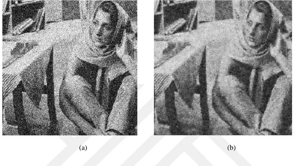
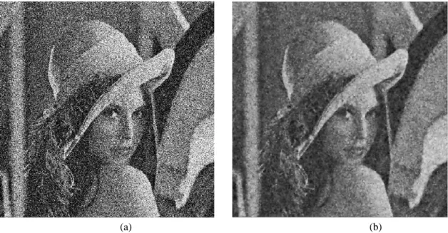
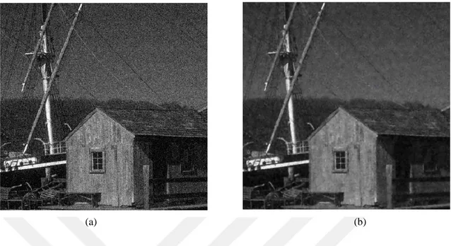
4.1. Results of circular wavelet de-noising by thresholding ... 40
4.1.1. Results of circular wavelet de-noising by thresholding ... 40
4.1.2. Circular wavelet results for images with salt and pepper noise ... 50
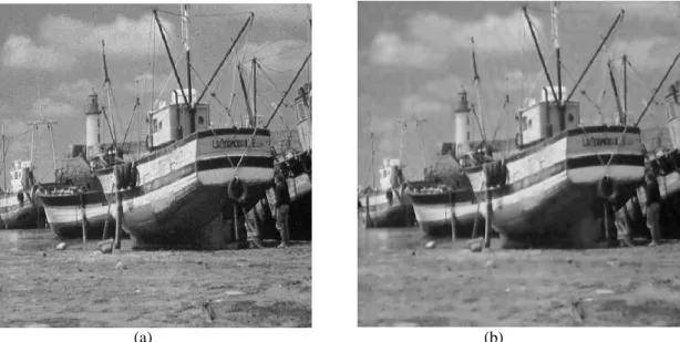
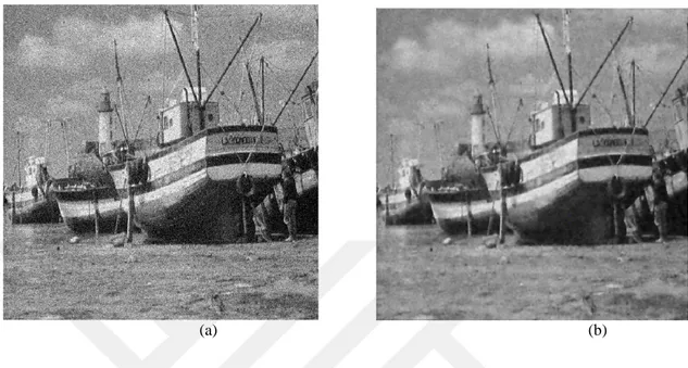
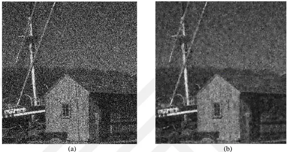
4.2. Results of Conventional wavelet de-noising by thresholding ... 60
4.2.1. Conventional wavelet Results for images with Gaussian noise ... 60
4.2.2. Conventional wavelet Results for images with salt and pepper Noise ... 70
4.3. A Comparative Study ... 70
5. CONCLUSIONS AND FUTURE WORK ... 73
5.1. Conclusions ... 73
5.2. Future Works ... 74
REFERENCES ... 75
VI
SYMBOLES AND ABBREVIATIONS Symbols
σ : Noise deviation
t : Predicted noise threshold level c(n,m) : Matched coefficient sub-symbol g(m,n) : Noise- clear image
Ψ(t) : Mother wavelet
X(f) : Signal fourier transform x(t)
L : Lemotes the number of decomdosition levels 𝛹𝑎,0(𝑡) : Time- scaled mother wavelet
𝛹𝑤 : Fourier transform
C : Admissibility constant 𝑋𝑊𝑇 : Continous wavelet transform
𝜓𝑗,𝑘(𝑡) : Discrete wavelet transform
𝐻𝑝(𝑧) : Equivalent representation of analysis 𝐹𝑝(𝑧) : Synthesis filter bank
𝐴(𝑧) : All-pass filter 𝐻0(𝑧) : Low- pass filter 𝐻1(𝑧) : High-pass filter
Abbreviations
PSNR : Peak signal noise ratio MAE : Mean square error MSE : Maximum signal error STFT : Short time fourier transform
WT : Wavelet transform
CWT : Continuous wavelet transform QMF : Quadrature mirror filter WDFS : Wave digital filters
LWDFS : Lattice wave digital filters
2
1. INTRODUCTION
1.1. Introductory Remarks
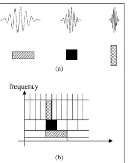
Images are often suffering from two main corruptions (unwanted modifications). These modifications in image accuracy are categorized as blur and noise. Blur is intrinsic to image acquisition systems, as digital images have a finite number of samples and must satisfy the Shannon-Nyquist sampling conditions (Buades et al., 2005). The second main image perturbation is noise. Image noise is random variation of brightness or color information in images, and is usually a result of some defects in the handling optical and electronic systems. Noise appears during different image processing phases of acquisition, transmission, and retrieval. The purpose of any de-noising algorithm is to remove such noise while maintaining as much as possible image details (Chen et al., 2006; Shinde et al., 2012). Since some fine details of the image always occupy the same high-pass spectrum, then they will be confused with the noise or vice-versa. The need of an image without noise is a requirement for many image processing algorithms such as pattern recognition, compression, etc. to efficiently work. Such requirements justify the importance of de-noising in images. Images can be affected by different types of noise sources. In a digital camera, noise may be added to the image while passing through lens, sensors, and ADC. In addition, the image processing block itself may add some noise. The types of image noise can range from salt and pepper, additive white Gaussian (AWG) to speckles (Verma and Ali, 2013).
In classical terms, the 1-D wavelet transform of Fig. 1.1 can be extended to 2-D wavelet transform. At each decomposition level, the 1-D transform is first applied across all the rows and then across all the columns to acquire a 2-D transform. At each decomposition level, four coefficients sets are produced: HH as the details across the diagonal direction, HL as the details across the vertical direction, LH as the details across the horizontal direction and LL as the average.
3
Fig. 1.1 1-D wavelet transform and it’s inverse. (a) 1-D wavelet 3-level decomposition (wavelet transform WT), (b) 1-D wavelet 3-level reconstruction (inverse wavelet transform IWT).
In 2-D case, the original image signal x(m, n) can be considered as if it is a combination of 1-D row signals and 1-D column signals. As it is done in 1-D case, each row of the image is processed first, in 2-D Discrete Wavelet Transform (DWT), then each column is processed. Figure 1.2 demonstrates a one-level image decomposition and reconstruction. In a similar way as in signal decomposition, the subsampling process is applied after each filtering. The whole process results in four sub-images, namely; approximation component and horizontal, vertical & diagonal details. The resulting sub-images have quarter the size of the original image, that because of the sub-sampling after each filtering.
a)
4
Fig. 1.2. One-level DWT steps of a 2-D image, (a) Decomposition, (b) Reconstruction.
A classical wavelet de-noising scheme is shown in Fig. 1.3, it consists of 2-D wavelet transform, 2-D inverse wavelet transform and an intermediate thresholding stage to shrink wavelet coefficients. In such thresholding stage, the level of the noise is first estimated and the appropriate thresholds are set. It should be noted that setting an appropriate value for the level of thresholding is an important point in thresholding. Recently, to calculate the value of thresholding, many approaches have been given. the estimation of the level of noise is needed by most of those approaches. Though, a useful tool for an estimator is the standard deviation of the data values. A good estimator
𝜎
for the wavelet de-noising is proposed by Donoho (Ergen, 2012) and given as;𝜎 =𝑚𝑒𝑑𝑖𝑎𝑛(𝑑𝐿−1,𝑘)
0.6745 , 𝑘 = 0,1, … , 2𝐿−1− 1 (1.1)
where L denotes the number of decomposition levels. The median selection is applied on the detail coefficient of the decomposed signal.
5
Fig. 1.3. Thresholding strategies, (a) Hard thresholding, (b) Soft thresholding.
Fig. 1.4. A classical scheme for wavelet de-noising.
In Fig. 1.3, the intermediate stage of wavelet coefficient shrinking (i. e., thresholding) can be performed either by hard thresholding or by soft thresholding strategies (as shown in Fig. 1.4). Generally, thresholding process will allow the detail coefficients which are greater than the threshold level to pass (i. e., considering them as image high frequency components) while preventing the lower level coefficients from passing through the threshold (i. e., considering them as noise components). The two strategies of thresholding are having many limitation and property considerations. Small changes in pixel level can usually very sensitive and unstable to the hard thresholding strategy. On other side, unnecessary level of level for true large coefficients can be occur on the soft thresholding strategy. Many sophisticated methods are proposed to overcome
6
the drawbacks of the thresholding described nonlinear strategies. Despite that, hard and soft thresholding are still applicable and treated as the most reliable and efficient thresholding techniques.
1.2. Aim of the Thesis
Proposing, constructing and testing a new image de-noising algorithm based on a 2-D CSWT. By using 2-D circular spectral split schemes with the efficient frequency-masking application for the realization of the designed 2-D circular wavelet filter bank branches, this 2-D CSWT is a geometrical image transform can be constructed. Via some metrics, the performance of the proposed system is to be tested. These metrics include correlation factor and Peak signal-to-noise ratio (PSNR) in dB.
1.3. Thesis Outline
In addition to this introduction in Ch.1, four other chapters are included in this thesis. Chapter 2 gives some fundamentals of wavelets and filter banks. Types of wavelet transform are also discussed. In addition, traditional FIR and IIR wavelet filter banks are included. Lattice wave digital filters (LWDFs) are introduced also for IIR filter bank simulation.
In Chapter 3, the proposed methodology is described. The idea of circular wavelet transform is introduced and some properties of such transform are highlighted. A de-noising diagram is proposed using the circular wavelet transform. A 3-decomposition level simplified de-noising structure is also derived with efficient realization.
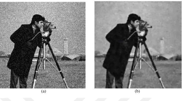
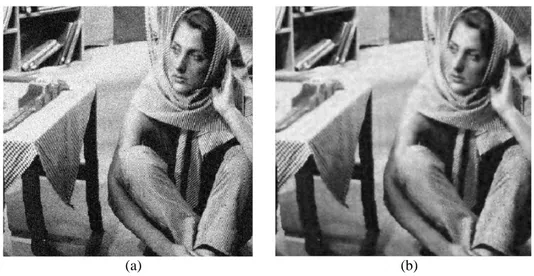
Chapter 4 contains the implementation and testing of the proposed methodology, showing some results highlighting the performance of the whole de-noising process. In such process, five standard images (including three different levels of two types of noise "Salt & pepper and Gaussian") are tested.
7
2. WAVELET FUNDAMENTALS AND LITERATURE REVIEW
Signal transformation is just another form of representing the signal, so that the information content present in the signal will not be changed. The wavelet transform (WT) is a very powerful transform, used in different branches of science. The power of the transform comes from the fact that the basis functions of the transform are localized in time and frequency with their different resolutions.
2.1. The Wavelet Transform
To overcome the shortcoming of the Short Time Fourier Transform (STFT), the wavelet transform was developed and in analyzing the non-stationary signals, it can be used.
Different frequencies are analyzed with different resolutions in the wavelet transform uses multi-resolution technique while the STFT gives a constant resolution at all frequencies. In a multi-carrier system, the wavelet transform can be used as a possible transform to generate sub-channels (Srivastava and Maheshwari, 2015).
As shown in Fig. 2.1, the wave is an oscillating function of time and is periodic, while wavelets are just localized small waves (Mastriani, 2015). The energy of wavelets can be concentrated in time and are suited for analyzing the transient signals. Fourier transform, STFT and wavelet transform are different. The sinusoidal waves to analyze signals are using in the first two types of transformation, while finite energy wavelets are using in the third to transfer the signals (Abdul-Jabbar et al., 2013).
(a) (b)
Fig. 2.1 Demonstration of (a) a Wave and (b) a Wavelet, (Srivastava and Maheshwari, 2015).
In the sense that the signal to be analyzed is multiplied with a wavelet function, the STFT analysis is also similar to the wavelet analysis, while it is only multiplied with
8
a window function in the STFT, and then at each segment generated the transform is computed. Also, in wavelet transform, the wavelet function width changes with each spectral component, while in STFT, the width of the window function is keeping constant. At high frequencies, it gives poor frequency resolution and good time resolution while at low frequencies, the wavelet transform gives poor time resolution and good frequency resolution (Abdul-Jabbar and Abdulkader, 2012; Srivastava and Maheshwari, 2015).
The wavelets are denoted to the functions generated from one single function (basis function) and this single function is called the mother wavelet. Other related wavelets contain dilations (scaling parts) and translations (shift parts) in time domain. The other wavelets
𝜓
a,b(t) can be represented as following while the mother wavelet isdenoted by
𝜓
(t):𝜓
𝑎,𝑏(𝑡) =
1
√|𝑎|
𝜓 (
𝑡 − 𝑏
𝑎
)
(2.1)where b and a are two random parameters. In the time axis, they denote the parameters for translations and dilations, respectively.
It is obvious from equation (2.1) that the mother wavelet can be essentially represented as
𝜓(𝑡) = 𝜓
1,0(𝑡)
(2.2)For a ≠ 1 and b = 0,
𝛹
𝑎,0(𝑡)
can be written as:𝛹
𝑎,0(𝑡) =
1
√|𝑎|
𝜓 (
𝑡
𝑎
)
(2.3)𝜓
a,0(t) As shown in equation (2.3) is a time-scaled mother wavelet𝜓(𝑡)
by afactor of a with amplitude-scaling by factor of
1/√|𝑎|
. a < 1 stands for time-compression while a > 1 reflects time-expansion. That’s the reason behind calling the parameter a as dilation (scaling) parameter. When a < 0, the function𝜓
a,b(t) results in9
As shown in the resulting wavelet function
𝜓
a,b(t) in eq. (2.1), the mathematicallysubstituting t in eq. (2.3) by t-b will cause a shift or translation in the time axis. The time axis right side will be shifted by a value of b as the function
𝜓
a,b(t) is a shifted version of𝜓
a,0(t) when b > 0 whereas, when b < 0, it is a shift in the time axis left side by a valueof b. Due to that the variable b will be representing the translation in time domain (shift in phase). In the time domain, the mother wavelet and its dilations will be illustrated as in Fig. 2.2 with the parameter of dilation a = α.
Fig. 2.2. (a) A mother wavelet
𝛙
( t ) , (b)𝛙
( t /α) :0 < α < 1, (c)𝛙
(t/α:): α > 1, (Abdul-Jabbar and Abdulkader, 2010).Fig. 2.2 (a) shows the mother wavelet
𝜓
(t) while a signal with compressed version in the axis of time when α < 1 is shown in Fig. 2.2 (b) and Fig. 2.2 (c) is showing the signal expansion in the axis of time when α > 1. The wavelet transform of the signal x(t) based on wavelets definition, can mathematically be represented by Abdul-Jabbar and Abdulkader (2010):𝑊(𝑎, 𝑏) = ∫ 𝑥(𝑡) 𝜓
𝑎,𝑏+∞
−∞
(𝑡)𝑑𝑡
(2.4)Mathematically, the reconstruction of x(t) from W(a,b) inverse transform is represented by:
10
𝑥(𝑡) =
1
𝐶
∫
∫
1
|𝑎|
2𝜓
𝑎,𝑏(𝑡) 𝑊(𝑎, 𝑏)𝑑𝑎 𝑑𝑏
+∞ 𝑏=−∞ +∞ 𝑎=−∞ (2.5) Where𝐶 = ∫
|ψ(𝜔)|
|𝜔|
2 +∞ −∞𝑑𝜔
(2.6)The Fourier transform of the mother wavelet
𝜓
(t) isψ(ω)
.W(a ,b) in equation (2.4) will be then named continuous wavelet transform (CWT), if x(t) b and a are continuous,. Hence the bi-variant function W(a, b) of two continuous real variables can be gotten from the CWT of a 1-D continuous function x(t), specifically; b as the translation and a as the dilation (Abdul-Jabbar and Abdulkader, 2010).
2.2. Conditions of Wavelets
if the following mathematical criteria are fulfilled, as a wavelet, an analyzing function
𝜓
(t) can be used:1- A finite energy must be in the wavelet i.e.,
𝐸 = ∫ |𝜓(𝑡)|
∞ 2−∞
𝑑𝑡 < ∞
(2.7)
the following condition must hold if
ψ (ω)
is the Fourier transform of the wavelet𝜓
(t),𝐶 = ∫
|𝜓̂ (𝜔)|
2𝜔
∞ 0𝑑𝜔 < ∞
(2.8)11
As per this condition, no zero-frequency component (
ψ
(0) = 0) will be on the wavelet, i.e., the wavelet𝜓
(t) mean must be equal to zero. Admissibility constant can be named to this condition. The chosen wavelet will be effecting the value of C.It is well known that wavelets can be classified into two classes: (a) orthogonal and (b) bi-orthogonal. Based on the application, either of them can be used (Shinde et al., 2012).
2.3. Types of Wavelet Transform
2.3.1. Continuous wavelet transform
The continuous wavelet transform (CWT) is normally represented by
𝑋
𝑊𝑇(𝜏, 𝑠) =
1
√|𝑠|
∫ 𝑥(𝑡) . 𝜓
∗
(
𝑡 − 𝜏
𝑠
) 𝑑𝑡
(2.9)with s=a and τ=b.
𝜓
∗: is the conjugate of ψ(t).where x(t) is the signal to be analyzed. ψ(t) is the mother wavelet or the basis function. A mother wavelet can generate all the wavelet functions that can be utilized in the transformation through translation (shifting) and scaling (dilation or compression) (Abdul-Jabbar and Abdulkader, 2012).
A limitation in STFT is the use of only one window size for all frequencies (see Fig. 2.3 (a)), so the resolution of the analysis in the time-frequency plane is unchanged at all locations as shown in Fig. 2.3 (b).
12
Fig. 2.3 Basis functions and time-frequency resolution of the short-time Fourier Transform (STFT). (a) Basis functions. (b) Coverage of time-frequency plane, (Daubechies, 1988).
In the WT, the time-frequency resolution is different from the STFT, where it is sharper in time at high frequencies, while it is sharper in frequency, at low frequencies, as shown in Fig. 2.4 (b). Such requirement just fits the physical properties of signals (Daubechies, 1988).
Fig. 2.4 Basis functions and time-frequency resolutions of the wavelet transform (WT). (a) Basis functions. (b) Coverage of time-frequency plane, (Daubechies, 1988).
13
2.3.2 Discrete wavelet transform
In continuous wavelet transform (CWT), the signals can be analyzed using a set of basic functions which are related to each other by simple scaling and translation. In the form shown so far, the difficulty of using directly properties can be within the CWT. That is the redundancy in the CWT. CWT is calculated by continuously shifting a continuously scalable function ψ(t) over the signal x(t) and calculating the correlation between the two. These scaled functions may not be orthogonal basis. Therefore, the obtained wavelet coefficients will be highly redundant. To overcome this problem, discrete wavelet transforms (DWT) is introduced. DWT is not continuously scalable and translatable but can only be scaled and translated in discrete steps. This is achieved by modifying the wavelet representation to
𝜓
𝑗,𝑘(𝑡) =
1
√𝑠
0𝑗𝜓 (
𝑡 − 𝑘𝜏
0𝑠
0 𝑗𝑠
0𝑗)
(2.10)j and k are integers and s0 > 1 is a fixed dilation step (Combes et al., 2012). The
translation factor τ0 depends on the dilation step. The sampling of the frequency axis
corresponds to dyadic sampling as the choosing of s0=2. It is usually selecting that τ0=1
for the translation factor, it will fulfill the achievement of the dyadic sampling of the time axis, yielding s=2j and τ=k 2j. Then it can be written that
𝜓
𝑗,𝑘(𝑡) = 𝜓
𝑠,𝜏(𝑡) =
1
√𝑠
𝜓 (
𝑡 − 𝜏
𝑠
)
(2.11)An infinite number of translations and scaling still be desirable even with discrete wavelets to compute the wavelet transform. By not to use an infinite number of discrete wavelets this problem will be processed. A band-pass like spectrum is seen in the wavelet. From Fourier theory, it is also known that compression in time is equivalent to stretching the spectrum and shifting it upwards. This means that a time compression of the wavelet by a factor of 2 will stretch the frequency spectrum of the wavelet by a factor of 2 and also shift all frequency components up by a factor of 2. Using this insight, the finite
14
spectrum of the signal which used in this thesis can be enclosed with the dilated wavelets spectra as shown in Fig. 2.5.
Fig. 2.5 Spectra of dilated wavelets, (Combes et al., 2012).
With a factor of two, every time in the time domain the wavelet is stretched and a half of the bandwidth is produced. In other words, half of the lasting spectrum with every wavelet stretch, is only covered, which indicates that to get the job done, an infinite number of wavelets is required.
With wavelet spectra, not to attempt to cover the spectrum all the way down to zero is basically the solution to this problem. Instead of that when it is small enough then use a cork to plug the hole. This cork then is a low-pass spectrum and it belongs to the so-called scaling function. Mallat (1989) is introduce this scaling function. it is sometimes denoted to as the averaging filter because of the low-pass nature of the scaling function spectrum. The stage of DWT analysis structure can then be reduced to a half-band two-branch filter bank which can be repeated, after down-sampling by 2, for many finite levels. A reversed structure with up-sampling by 2 and phase reversed filters can be used for the stage of synthesis. In the case of DWT, digital filtering techniques are used to obtain a time-scale representation for digital signal. The signal can be analyzed by passing it through filters with different cut-off frequencies at different scales (Combes et al., 2012). In numerous practical problems, the discrete nature of the signal that should be analyzed, announces the need to discretize the wavelet transform to use it for sampled discrete signals. Such discretization of the wavelet transform can be met efficiently, by applying recursive filtering stages in iterated filter-banks as shown in Fig. 2.6.
15
Fig. 2.6 Two-channel quadrature mirror filter banks, (Akansu and Haddad, 2001).
2.4 The Filter Bank
A pair of low-pass and high-pass half-band filters, which satisfy some complementary properties, can compose two-channel filter bank. Each of the two channel signals bandwidth is a half of the bandwidth of the original signal. From this, a half of the original signal sampling rate will be the sampling rate to process the channel signals. A down sampling by two for the channel signals at the output of the analysis bank, and then managed at the lower rate of sampling. Each of the two channel signals must be at start up sampled by two at the signal reconstruction, and then applied to process in the synthesis part of the filter bank.
Two unwanted effects can be caused from the conversion for the sampling rate in the two-channel filter bank: the first from down sampling the aliasing can be resulted, and the second from up-sampling is the imaging can be resulted. Auspiciously, in the synthesis part it can eliminate the aliasing resultant in the analysis part. in the analysis and synthesis part of the two-channel filter banks, choosing the proper combination of filters will achieve that. After eliminating the aliasing effect, the possibility of the nearly perfect (and perfect) reconstruction (NPR and PR) of the original signal can be understood. The perfect reconstruction means that the signal at the output of the filter bank is a delayed replica of the original input signal. The tree-structures where the two-channel filter bank is used as a building block are can be from the widely used and important structures for the two-channel filter banks. In this way, either uniform or non-uniform separation between the channels can give a multi-level multi-channel filter bank (Daubechies, 1988).
16
Selection of the filter that can be used in discrete wavelet filter banks is the most important role when designing it. Therefore, orthogonal and bi-orthogonal filters is the category of the filter banks types. Symlets, Coiflets, Daubechies and the other of derived FIR wavelet filters, are of perpendicular class. However, these filters are not symmetric and the perpendicular wavelet filters coefficients are real numbers. The high-pass and the low-pass filters do not have the same length in bi- perpendicular FIR wavelet filters, (such as bi- perpendicular 9/7 and bi- perpendicular 5/3). The high-pass filter could be either asymmetric or symmetric while the low-pass filter is always symmetric. The filters coefficients are either integers or real numbers and, a bi-orthogonal filter bank has all even length or all odd length filters, for perfect reconstruction (Chui, 2016).
2.4.1 Quadrature mirror filter (QMF) banks
For many communication and signal processing systems, quadrature mirror filter (QMF) banks have been widely used to realize the goals of sub-band coding and short-time spectral analysis. The QMF bank is used to decompose a signal into sub-bands. These sub-band signals in the analysis system are then decimated by an integer equal to the number of sub-bands. Furthermore, two-channel QMF banks can be used easily for constructing M-channel QMF banks based on a tree structure (Chui, 1992). The two-channel QMF banks, as shown in Fig. 2.6, have received a great interest because of a wide variety of engineering applications. A common requirement in most applications is that the reconstructed signal should be as close to the input signal as possible. In general, the reconstructed signal suffers from three types of error: aliasing error, amplitude distortion, and phase distortion. One of the purposes of QMF designs is to eliminate these three distortions so that the reconstructed signal becomes the exact replica of the original signal with some delay. This is known as perfect reconstruction condition (Akansu and Haddad, 2001).
2.4.2. The analysis and the synthesis filter banks
Analysis filter bank is used to decompose an input signal into sub-bands of the frequency. The two-channel analysis filter bank is shown in Fig. 2.7. Firstly, by passing such X(z) through a high-pass filter H1(z) and low-pass filter H0(z) to produce the U0(z)
17
U0(z) and a high frequency component U1(z) are split (Vaidyanathan, 1993; Fliege, 1994;
Strang and Nguyen, 1996).
Fig. 2.7 Two-channel analysis filter bank, (Vaidyanathan, 1993).
Accordingly, the available bandwidth from 0 to π with the sampling frequency, 𝜔s = 2π, is divided into two halves, π /2 ≤ 𝜔 ≤ π for the high frequency spectrum U1(z)
and 0 ≤ 𝜔 ≤ π /2 for the lower frequency spectrum U0(z). Thus, after being passed through
the high-pass filters and low-pass respectively, the filtered spectra U1(z) and U0(z) passes
half the input signal bandwidth. Fig. 2.8 shows the down sampled and filtered signal spectra.
18
On the other side, a two-channel synthesis filter bank, shown in Fig. 2.9, contains up-samplers by two to produce signal spectrums U0(z) and U1(z). The next step is passing
these spectrums through G1(z) and G0(z) that denote both high-pass and low-pass filters,
and then recombining the up-sampled spectrums U1(z) and U0(z) into input signal
reconstructed version
𝑋̂(𝑧)
i.e., the same as the input signal with some delay for perfect reconstruction property (Vaidyanathan, 1993).Fig. 2.9 Two-channel Synthesis filter bank, (Vaidyanathan, 1993).
2.4.3. The perfect reconstruction conditions for QMF banks
The analysis and synthesis filters must undertake certain conditions to realize the perfect reconstruction. Let H0(z) and H1(z) be the low-pass and high-pass analysis filters,
respectively and G0(z) and G1(z) are the low-pass and high-pass synthesis filters,
respectively.
The synthesis filters G0(z) and G1(z) can be obtained depending on the following
QMF bank conditions: H1(z)=H0(-z), G0(z)=H0(z) and G1(z)=-H0(-z), that because of
existence of the mirror image symmetry (about the frequency ω=π/2) between H0(ejω) and
H1(ejω) as shown in Fig. 2.10 (Vaidyanathan, 1993).
19
To achieve both perfect reconstruction and orthonormality properties, the analysis and synthesis filters must satisfy the following two conditions (Akansu and Haddad, 2001; Srivastava and Maheshwari, 2015):
𝐻
0(−𝑧)𝐺
0(𝑧) + 𝐻
1(−𝑧)𝐺
1(𝑧) = 0
(2.12)and
𝐻
0(𝑧)𝐺
0(𝑧) + 𝐻
1(𝑧)𝐺
1(𝑧) = 2𝑧
−𝑙 (2.13)The first condition represents that the amplitude distortion has a maximum amplitude of one and the second condition represents that the reconstruction is an aliasing-free one. The above conditions can be satisfied in many filters. But especially when the filter coefficients are quantized, accurately wavelet transforms cannot be achieved from all of them. After the reconstruction by calculating the SNR of the signal, the accuracy of the wavelet transform can be determined (Srivastava and Maheshwari, 2015).
2.5 Filter Bank for Discrete Wavelet Transform
In signal processing functions, the most widely used applications is filters. Wavelets can be realized by iteration of filters with rescaling. The resolution of the signal, which is a measure of the amount of detail information in the signal, is determined by the filtering operations, and the scale is determined by up-sampling and down-sampling operations (Akansu and Haddad, 2001).
The DWT can be computed by using consecutive low-pass and high-pass filtering of the discrete time-domain signal as shown in Fig. 2.11. In such figure, the input signal is denoted by the sequence x(n), where n is an integer. The low-pass filter is denoted by H0 while the high-pass filter is denoted by H1. At each level, the high-pass filter produces
detail information, di(n), where i is the level number. rough approximations, ai(n) and be
earned from the association of scaling function with low-pass filter (Vaidyanathan, 1993; Fliege, 1994; Strang and Nguyen, 1996).
20
Fig. 2.11 Three-level wavelet decomposition tree, (Vaidyanathan, 1993).
At each decomposition level, the half-band filters produce signals spanning only half the frequency band for the previous level signal. The uncertainty in frequency is reduced by half in other word, this doubles the resolution of the frequency. If the original signal has a highest frequency of B and accordanly to Nyquist’s rule, which needs a sampling frequency of 2B radians, then it owns now after passing through filters level one, a highest frequency of B/2 radians. With the removal of half of the samples number without loss of information at a frequency of B radians, it can now be re-sampled. This is called decimation by 2 which halves the time resolution as the entire signal is now represented by only half of the number of samples. Consequently, the half band low-pass filtering removes half of the frequencies and thus halves the resolution. So the decimation by 2 doubles the scale.
The filtering and decimation processes are continued until the desired level is reached. The length of the signal always determines the maximum number of levels that is needed. The DWT of the original signal is then obtained by concatenating all the coefficients, ai(n) and di(n), starting from the last level of decomposition.
The structure of reconstruction of the original signal from the wavelet coefficients is shown in the Fig. 2.12. Principally, the reverse process of decomposition is the reconstruction. At every level the detail coefficients and approximation are up-sampled by 2, passed through the high-pass and low-pass combination filters and then summed. As in the process of the decomposition, this process is sustained through the same number of levels to gain the original signal. If the analysis filters, H1 and H0, are exchanged with
the combination filters, G1 and G0, the Mallat algorithm functions equally positive
21
Fig. 2.12 Three-level wavelet reconstruction tree, (Vaidyanathan, 1993).
2.6. Traditional Structures for Discrete Wavelet Transform
There are a variety of structures to implement a filter bank. The followings represent the traditional structures for DWT filter banks (Shukla and Tiwari, 2013):
1) structure of Direct form. 2) structure of Lifting scheme. 3) structure of Lattice.
4) structure of Poly phase.
2.6.1. Direct form structure
The structure of direct form can be divided into two parts: followed by decimators, the first part is analysis filter having high-pass and low-pass filters. The second part is the synthesis filters containing up-samplers followed by the low-pass and high-pass filters as shown in Fig. 2.6 (Akansu and Haddad, 2001).
2.6.2. Poly-phase structure
The input signal is split into even and odd samples in the poly-phase form (decimation by 2 is automatically in the input), correspondingly, a split into odd and even components in filter coefficients are also happen so that Xodd convolves with H0odd of the
22
output, the two phases are summed together. For the high-pass filter, the same method is applied where the high-pass filter is split into even and odd phases H1even and H1odd. The
poly-phase analysis operation can be represented by the following matrix equation:
[
𝐻
𝐻
0𝑒𝑣𝑒𝑛𝐻
0𝑜𝑑𝑑 1𝑒𝑣𝑒𝑛𝐻
1𝑜𝑑𝑑] × [
𝑋
𝑒𝑣𝑒𝑛𝑍
−1𝑋
𝑜𝑑𝑑] = 𝐻
𝑝(𝑧) [
𝑋
𝑒𝑣𝑒𝑛𝑍
−1𝑋
𝑜𝑑𝑑] = [
𝑌
0𝑌
1]
(2.14)In eq. (2.14), the sub-filter H0even and H0odd possess half of the length of the filter
H0, So, the even and odd terms are filtered separately by the even and odd coefficients of
these sub-filters. Such sub-filters can operate in parallel to improve speed efficiency. Fig. 2.13 illustrates analysis and synthesis part for poly-phase filter banks (Srivastava and Maheshwari, 2015).
(a)
(b) (c)
Fig. 2.13 structure of Poly-phase of (a) analysis filter bank (b) equivalent representation of analysis filter bank and (c) synthesis filter bank, (Akansu and Haddad, 2001).
23
𝐻
𝑝(𝑧) = [
𝐻
𝐻
𝑜𝑒𝑣𝑒𝑛(𝑧) 𝐻
0𝑜𝑑𝑑(𝑧)
1𝑒𝑣𝑒𝑛(𝑧) 𝐻
1𝑜𝑑𝑑(𝑧)
]
(2.15) and𝐹
𝑝(𝑧) = [
𝐺
𝐺
0𝑒𝑣𝑒𝑛(𝑧) 𝐺
1𝑒𝑣𝑒𝑛(𝑧)
0𝑜𝑑𝑑(𝑧)
𝐺
1𝑜𝑑𝑑(𝑧)
]
(2.16) 2.6.3 Lattice structureHP(z) can be replaced by a structure of lattice in the poly-phase matrix of eq.
(2.15). If the filters H1(z) and H0(z) are identified, the filter bank, HP(z) can be gained.
Correspondingly, the structure of lattice can be derived by representing it as a product of simple matrices, if HP(z) is known. FIR wavelet filter banks can have competently
structures of lattice which are easy to implement.
The structure of lattice decreases the multiplications number by reducing the number of resulting coefficients. The structure consists of some design parameters ki that
can be calculated from the FIR filter function and a single overall multiplying factor M. Fig. 2.14 shows the complete structure of lattice for an orthogonal FIR filter bank (Verma and Ali, 2013; Srivastava and Maheshwari, 2015).
Fig. 2.14 Lattice structure of an orthogonal FIR filter bank, (Fliege, 1994).
2.6.4. Lifting scheme structure
The lifting scheme is shown in Fig. 2.15. It is proposed independently by Herley and Swelden which consists of two steps: dual lifting and lifting step. This structure can be considered the efficient method to construct two-channel filter banks and the fast.
24
Fig. 2.15 Lifting scheme implementation, (Fliege, 1994).
By using this method, filters with positive properties which fulfill the perfect properties of reconstruction can be built (Akansu and Haddad, 2001). A non-traditional structure is to be designed and implemented in this work utilizing IIR filter banks with lattice all-pass sections.
2.7. All-Pass Filters
In digital signal processing the useful building blocks are all-pass filters that have a nonlinear phase characteristic to construct efficient IIR systems. An all-pass filter A(z) is a system having a constant magnitude response for all the frequencies, i.e.,
|𝐴(𝑒
𝑗𝜔𝑡)| = 𝑐,
𝑓𝑜𝑟 𝑎𝑙𝑙 𝜔.
(2.17)c: constant.
the group delay distortion or phase equalization without affecting the magnitude response is a strong application of all-pass networks with unit magnitude response. In particular, an important increase of the group delay in the near of the cutoff frequencies can be given from the classical IIR filters. To add extra delay in those frequency ranges is the equalization meaning in this context, where the given characteristic of delay shows low values. The resulting group delay response should be as flat as possible in the pass-band of the filter, so that the signal shape in the time domain can be preserved (Akansu and Haddad, 2001).
The transfer function of an Nth -order all-pass filter will be stated in the product form as shown in the following equation:
25
𝐴(𝑧) = ∏
𝑧
−1− 𝑎
𝐾∗1 − 𝑎
𝐾𝑧
−1 𝑁 𝐾=1 (2.18)where ak, k = 1, 2, …, N, is a complex number representing the pole of A(z). It is clear
from eq. (2.18) that the poles and zeros of the transfer function are reciprocal to each other. To satisfy the stability condition, the poles should be placed inside the unit circle, and consequently the module of ak is limited with |ak| < 1. Automatically, the transfer
function zero being reciprocal to the poles must place out of the unit circle. In fact, by reversing the order of the coefficients, the numerator polynomial can be obtained from the denominator polynomial. For example, a second -order all-pass filter can be represented by the following transfer function (Akansu and Haddad, 2001):
𝐴
𝐴𝑃(𝑧
2) =
𝑎
2+ 𝑎
1𝑧
−1+ 𝑧
−21 + 𝑎
1𝑧
−1+ 𝑎
2𝑧
−2(2.19)
2.8. FIR and IIR Wavelet Filter Banks
The FIR wavelet filters are usually utilized in the design of the wavelet filter banks, but it is well known that these filters haven’t high frequency discrimination. To increase the discrimination properties for such FIR filters, their order must be increased, but this will in turn increase the implementation complexity and time delay. As a solution, the highly discriminative IIR wavelet filter banks that have less implementation complexity and less time delay which can be proposed instead of the classical FIR wavelet filter banks.
Recursive filter algorithms are required to realize such IIR filters. A class of recursive filters that can be implemented with a guaranteed stability is wave digital filters (Akansu and Haddad, 2001).
2.8.1. Two-channels QMF banks using all-pass filters
It has been shown that using a two-channel QMF banks can eliminate both aliasing error and amplitude distortion completely. The IIR wavelet filter banks can be designed composing two all-pass filters (this circuit is considered as the best kernel for building up
26
a multi-channel IIR filter banks). Fig. 2.16 shows the based IIR QMF banks two-channel all-pass filter (Akansu and Haddad, 2001).
Fig. 2.16 Lattice structure realization of the IIR wavelet filter bank. (a) Direct lattice structure realization. (b) Computationally efficient realization, (Akansu and Haddad, 2001).
A branch-interchange method is applied in the two all-pass sections of analysis and synthesis sides to remove the phase distortion (Akansu and Haddad, 2001). As shown in Fig. 2.17 a modified stable linear phase structure can also be derived.
Fig. 2.17 The modified lattice structure realization of the IIR wavelet filter bank, (Akansu and Haddad, 2001).
27
In this work, the design of two-channel linear-phase QMF banks constructed using real IIR digital all-pass filters is considered. The design problem is appropriately formulated to result in a simple optimization problem. Using both intermediate filter design and Gazsi method (Abdul-Jabbar, 2011), to find the real coefficients for the IIR digital all-pass filters, the optimization problem can be efficiently solved through equating the numerator of the transfer function of the bi-reciprocal lattice wave digital filter with the numerator that resulting from the transfer function of intermediate filter. The resulting two-channel QMF IIR filter banks possess approximate linear-phase response without magnitude distortion; that is the main advantage of using all-pass sections (Chui, 1992).
2.8.2 IIR wavelet filter banks
When using lattice structure with all-pass sections of the types shown in Figs. 2.16 and 2.17, a all-pass filter-based IIR QMF banks with two-channel can be represented by a very efficient way. In Fig. 2.16 the components of lattice are the second-order all-pass filters A0(z2) and A1 (z2) with the following transfer functions (Akansu and Haddad, 2001):
𝐴
0(𝑧
2) = ∏
𝛼
𝑖+ 𝑧
−21 + 𝛼
𝑖𝑧
−2 (𝑁+1)/2 𝑖=2,4 (2.20) And𝐴
1(𝑧
2) = ∏
𝛼
𝑖+ 𝑧
−21 + 𝛼
𝑖𝑧
−2 (𝑁+1)/2 𝑖=3,5 (2.21)where
𝛼
𝑖 is the multiplier coefficient value in the𝑖
th all-pass section.Let G1(z) and G0(z) denote the transfer functions of the high-pass and low-pass filter of
the combination part and let H1(z) and H0(z) denote the transfer functions of the high-pass
and pass filter of the analysis part of the QMF bank with two-channel. For the low-pass side, the analysis filters H1(z) and H0(z) can be written as (Akansu and Haddad,
2001):
𝐻
0(𝑧) =
1
2
[𝐴
0(𝑧
2) + 𝑧
−1𝐴
1(𝑧
2)]
(2.22)28
𝐻
1(𝑧) =
1
2
[𝐴
0(𝑧
2) − 𝑧
−1𝐴
1(𝑧
2)]
(2.23)2.9. Wave Digital Filters (WDFs)
Wave digital filters (WDFs) are well known to have many advantageous properties. Such properties include low coefficient sensitivity, good dynamic range, and especially, good stability properties, under different quantization levels (Shukla and Tiwari, 2013). WDFs comprise a eclectic class of IIR digital filters that are well appropriate for implementation. The lattice wave digital filter is the most attractive one among different wave digital filters. All WDFs have their corresponding filters in the analogue reference domain. Inherit of several fundamental properties, WDFs are derived from analog reference filters. If the reference filter has a low sensitivity to variation in element values, which is the case for certain RLC filters, the digital filter can be inherit this property (Shukla and Tiwari, 2013). One more property inherited from the reference filter is the stability for the filter through implementation. Richards’ structures and ladder structures are examples of structures of WDF, fitting for implementation. Though, lattice WDFs (LWDFs) is a class of WDFs that is even more suitable for VLSI implementation. From analog lattice filters, these filter structures are derived.
The type of IIR filters that well suit the implementation on FPGA is the lattice wave digital filter (LWDF) (Shukla and Tiwari, 2013).
2.9.1. Lattice wave digital filters (LWDFs)
Where each branch realizes an all-pass filter, an LWDF is a parallel structure of two-branch as shown in Fig. 2.18. There are several methods to appreciate LWDFs. One of the most striking method, as shown in Fig. 2.19, is to use cascaded first-order and second-order sections. By using symmetric parallel adaptors or two-port series, the second-second-order and first-order sections are realized with certain equivalence transformations. By using three-port series- or parallel adaptors, the second-order sections can also be realized (Abdul-Jabbar, 2009; 2011).
29
Fig. 2.18 Lattice wave digital filter block diagram, (Abdul-Jabbar, 2009).
Fig. 2.19 An 11th-order lattice wave digital filter (Abdul-Jabbar, 2009).
The LWDF structure inherits some properties from the reference filter (the analog lattice filter), the low-pass-band sensitivity and high stop-band sensitivity. The LWDF structure is well appropriate for VLSI implementation because it is highly modular yielding a high degree of parallelism. By using symmetric two-port adaptors, the all-pass filters are composed of cascaded second-order and first-order Richards’ structures implemented. The signal-flow graph of the symmetric two-port adaptor is shown in Fig. 2.20 (Abdul-Jabbar, 2009; 2011).
30
Fig. 2.20 A symmetric two-port adaptor, (Akansu and Haddad, 2001).
2.9.2. Bi-reciprocal lattice wave digital filters (BLWDFs)
A sub-class of LWDFs is bi-reciprocal LWDFs (BLWDFs). The magnitude function of a BLWDF is anti-symmetric around π/2. Comparing the BLWDF to the LWDF of the same filter order, more than half of the coefficients of the first are zeros (Abdul-Jabbar, 2009). Fig. 2.19 (for an 11th -order structure) can then be modified to BLWDF structure as shown in Fig. 2.21. This conversion will reduce the arithmetic complexity of the BLWDF implementation as well as increase the throughput, compared to an LWDF implementation (Abdul-Jabbar, 2011). Moreover, when the application is in a decimator or interpolator by a factor of 2, the filter can run at the lower sampling rate (Abdul-Jabbar, 2009).
31
The transfer function to the low-pass filter of a bi-reciprocal LWDF can be written as (Johansson and Wanhammar, 1996; Abdul-Jabbar, 2009):
𝐻(𝑧) =
1
2
[𝐴
0(𝑧
2) + 𝑧
−1𝐴
1(𝑧
2)]
(2.24)where the transfer function A0(z2) corresponds to the lower branch in Fig.(2-22) while
A1(z2) corresponds to the upper (Abdul-Jabbar, 2009).
The frequency response of the filter can be written as
𝐻(𝑒
𝑗𝜔𝑇) =
1
2
(𝑒
𝑗𝛷0(𝜔𝑇)+ 𝑒
𝑗𝛷1(𝜔𝑇))
(2.25)Where
𝛷
𝑘(𝜔𝑇) = −𝑘𝜔𝑇 + 𝑎𝑟𝑔{𝐻
𝑘(𝑒
𝑗𝜔𝑇)},
𝑘 = 0,1
(2.26)is the phase response of the kth branch and T is the sampling period. The magnitude of the overall filter is hence restricted by
|𝐻(𝑒
𝑗𝜔𝑇)| ≤ 1
(2.27)The BLWDF transfer function and its complementary transfer function are power complementary functions. So, BLWDFs have the following relationships:
|𝐻(𝑒
𝑗𝜔𝑇)|
2+ |𝐻(𝑒
𝑗(𝜔𝑇−𝜋))|
2= 1
(2.28)which means that the pass-band and stop-band edges (ωc & ωs, respectively) are related
by ωcT + ωsT = π.
to define the principles of the transmission zeros and the attenuation zeros, the following discussions are achieved. On the unit circle in the z-plane, these zeros always arise. Which the magnitude function reaches to its maximum value, an attenuation zero represents to an angle ω0T at. In the BLWDFs this takes place when
32
|𝐻(𝑒
𝑗𝜔0𝑇)| = 1
(2.29)At which the magnitude function is zero, a transmission zero represents to an angle ω1T
, i.e., when
|𝐻(𝑒
𝑗𝜔1𝑇)| = 0
(2.30)It follows from eq. (2.27) if the filter has an attenuation zero at ω0T, then that it also has
a transmission zero at π – ω0T.
The phase manners of an ideal poly-phase network must approximate the phase responses of the overall branch transfer functions to get a low-pass filter. The phase responses of both branches must have the same value at an attenuation zero, , i.e.,
𝛷
0(𝜔
0𝑇) = 𝛷
1(𝜔
0𝑇)
(2.31)Hence, the phase responses must be approximately equal in the filter pass-band. the difference in phase between the two branches must be at a transmission zero
𝛷
0(𝜔
1𝑇) − 𝛷
1(𝜔
1𝑇) = 𝜋
(2.32)Thus, the difference in phase between the two branches must approximate π in the stop-band of the filter. the degrees of A0(z2) and A1(z2) must differ only by one to make sure
that only one stop-band occur and one pass-band, (Abdul-Jabbar, 2009).
2.10. Literature Review
Many attempts were accomplished to de-noising noisy images, resulting in a wide variation in the output de-noised image performances.
In 2007, By using lifting schemes architectures for 2-D and 1-D discrete wavelet transform (DWT) were presented (Xiong et al., 2007). To optimize the architecture for 1-D 1-DWT, an embedded decimation technique was exploited, which was designed to receive an input and generate an output with the low- and high-frequency components of original data being available alternately. By employing parallel and pipeline techniques, based on the 1-D DWT lifting scheme architecture was extended to an efficient line-based architecture for 2-D DWT. Such techniques were mainly composed of one vertical filter
33
module and two horizontal filter modules, working in parallel and pipeline fashion with 100% hardware utilization. Two 2-D fast architectures were presented. They can perform J levels of decomposition for (N * N -sized) image in approximately 2N2(1 - 4(-J))/3 internal clock cycles. In tradeoff among hardware cost, throughput rate, output latency and control complexity, the lifting scheme architectures for 2-D DWT were proved to be efficient alternatives, compared with some other works reported in previous literature,.
In many other wavelet-based techniques, it has been proved that these techniques can offer good processing quality and best flexibility for the problem of noise in both 1-D signals & 2-1-D images. Noise-existence in image processing and applications is practically one of the most important problems to solve because it affects the overall performance of the imaginary systems. Therefore, various methods were developed by Turkish authors for de-noising. In 2007, Vatansever et al. (2002) presented a comparison of some wavelet de-noising methods with some recent methods, highlighting some of wave transform properties. Also in 2007, M. İkiz et al. (2007) suggested a classification system used to recognize the speaker identity by means of wavelet analysis and neural network approach. After sampling, the 1-D voice signals generated from 10 different persons (6 males and 4 females) were de-noised using Wave-flow and Wave-pad shareware programs. A Matlab Simulink model was designed to generate the tested data from the voice signals. This data was applied once again as an input signal for a Matlab-based neural network to classify the voice data into different speakers. Again in 2007, Demir and Erturk (2007) proposed a hyperspectral image classification approach using support vector machines (SVM) after a wavelet de-noising. The noise reduction was carried out in each band independently. Compared with direct SVM based classification, it was shown that the SVM classification of de-noised images can result in significantly better classification accuracy, improved sparsity and faster testing time. Such properties make the wavelet de-noised SVM based hyperspectral classification approach more suitable for low-complex and real-time applications.
In 2010, based on the Haar wavelet transform a de-noising algorithm was presented by a non-Turkish. By using the Tetrolet transform the methodology was based on an algorithm initially developed for compression of image. An adaptive Haar wavelet transform whose support is tetrominoes that is basically called The Tetrolet transform, that is, shapes made by connecting four equal sized squares. By an additive white Gaussian noise (AWGN) with the assumption of universal hard thresholding, and over the classical Haar wavelet transform, that algorithm gave 2.5 dB improvement in PSNR
34
for some de-noised test images corrupted previously. By such algorithm, on each 4x4 block of the image, it had been shown that the algorithm was local and can work independently. In addition, the algorithm was well suited for efficient hardware implementation because of its local nature and the simplicity of its computations (Singh, 2010).
Back to Turkish authors, Ergen and Baykara (2011) gave a comparison between the wavelet and wavelet package decomposition for image de-noising. They examined many standard test images and their results showed that increasing of decomposition depth has no effect on improving the values of peak signal- to-noise ratio (PSNR). They concluded that wavelet decomposition is superior to wavelet package decomposition and more suitable to be used in image de-noising. In addition, the performances of wavelet de-noising methods were examined in 2012 by Ergen (2012) for several variations including various rules of thresholding with different types of wavelet filters. Comparisons were accomplished for the three estimation methods of threshold with different wavelet types. Results have shown that rather than the wavelet type, the most important controlling factor in wavelet de-noising is decomposition level. It has been shown that neither the estimation of threshold value nor the threshold type has any effect on the de-noising quality. However, no worthy differences in the resulting de-noised images were seen till the 6-level decomposition, after such level, a better performance in terms of SNR level for Rigresure method was achieved over the others. Also, it was shown that the decomposition level was absolutely dependent on the frequency band of the image to be analyzed and its sampling frequency and for large oscillation numbers the wavelet type was not very important. one of the major application areas of communication systems is constituted in Radar. The noise may be mixed with the original signal because of human-induced or environmental reasons, while radar signal passes from source to target. Hence, it may be impossible to read the radar signal correctly because of that noise. a non-traditional wavelet packet transform (WPT) for the de-noising of weak radar signals with high-performance has been suggested in 2014 by Üstündağ et al. (2014). By applying the genetic algorithm (GA) structure as an intelligent system for optimization the appropriate wavelet family type while such non-traditional WPT transform were performed, decomposition level number and entropy type were instantaneously selected. Furthermore, by using the fuzzy s-function as a thresholding function and variable parameters of this function were set according to the best performance criteria, the suitable threshold function was selected. in the literature for de-noising of the weak radar
35
signals, the method was then compared with other algorithms available. Using root mean square error and the correlation coefficient criteria as metrics, the system performance was tested. Results highlighted that the suggested method gave better performance evaluations than the other de-noising methods available in the literature. Recently, in 2015, Srivastava and Maheshwari (2015) presented a work that reviewed and summarized the use of wavelet transform for de-noising of signals contaminated with noise. Their work also discussed the diverse applications of the wavelet transform.
With special emphasis in image de-noising in non-Turkish paper, Mastriani (2015) presented quantum Boolean image processing methodology. Two new interfaces of an approach for internal image representation was highlighting and presented: quantum-to-classical and classical-to-quantum. Working exclusively with computational basis states (CBS) the image de-noising was called quantum Boolean mean filter. The image was decomposed into its three color components (red, green and blue) in that sense. Then, for each color (with 8 bits per pixel), the bit-planes were obtained, i.e., 8 bit-planes per color. By using the most significant bit (MSB) bit-plane of each color, exclusive manner, all operations were accomplished. a quantum Boolean version of the image was achieved within the quantum machine, after a classical-to-quantum interface (which included a classical inverter). The methodology prevented the problem of quantum measurement, which alters the results of the measured except in the case of CBS. By proceeding to reassemble each color component, the results of filtering the inverted version of MSB, inside quantum machine, were passed through a quantum-to-classical interface (which involves another classical inverter). Finally, by filtering the image and discussing some appropriate metrics for image de-noising in a set of experimental results, this processing methodology was concluded. Such metrics include the correlation factor and Peak signal-to-noise ratio (PSNR). It had been shown that the results of such quantum Boolean de-noising methodology were superior to those obtained by the classical techniques.
36
3. THE PROPOSED METHODOLOGY AND EFFICIENT REALIZATION
In this chapter, a two-dimensional (2-D) circular-support wavelet transform (2-D CSWT) is introduced. A 2-D CSWT is simulated in forms of 2-D frequency- mask filter bank and introduced for de-noising of noisy images. A de-noising scheme via frequency masking realization of the overall filter bank is presented. Then, such overall structure is modified into some efficient one.
3.1. 2-D Circular-Support Wavelet Transform (2-D CSWT)
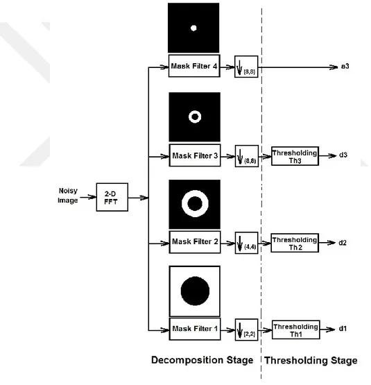
The 2-D CSWT is a geometrical image transform which was presented recently in 2013, Abdul-Jabbar et al. (2013) depending on the idea of 2-D elliptical–support wavelet filter bank (Abdul-Jabbar and Abdulkader, 2012). 2-D CSWT can efficiently represent images using 2-D circular spectral split schemes (circularly-decomposed frequency subspaces (Abdul-Jabbar and Abdulkader, 2010)). The classical one-dimensional (1-D) analysis Haar filter bank branches which are simulated as a parallel connection of both low-pass and high-pass filters, can be transformed into their 2-D counterparts. The designed 2-D circular wavelet filter bank branches can be easily realized by their frequency-masks. The proposed scheme consists of two parts as in the Figs. 3.1 and 3.2. They can be simulated using a Matlab program to obtain the low and high frequency coefficients (on two separable 2-D regions). As shown in the Fig. 3.1, a 3-level (or even more) 2-D circular decomposition stage with down-sampling by (2, 2) can be achieved, resulting in reducing the scales of the 2-D circular-splitting regions by a quarter at each decomposition scale. The input noisy image is decomposed by such 2-D CSWT transform into (r + 1)low- and high-pass coefficients, where r is the number of the decomposition level.
3.2. 2-D Circular-Support Wavelet Transform for Image De-noising
For the process of image de-noising, the decomposition stage of the 2-D CSWT can be adopted (as shown in Fig. 3.1) with some thresholding processes being applied on all high-pass coefficient channels. Different thresholding levels (Th1, Th2, and Th3) can be applied to maintain as much as possible noise-free high-pass channels.
37
Fig. 3.1 3-level decomposition stage of the proposed de-noising scheme with thresholding.
The de-noised image can result from the 2-D circular-support reconstruction filter bank which is shown also in the Fig. 3.2 as a reconstruction stage of the 2-D CSWT. In this stage, up-sampling by (2, 2) can be applied at each level to have the same size of the original image at the output.
38
3.3. Efficient and Simplified Structures
Some efficient and simplified structures of the 3-level 2-D circular decomposition and reconstruction stages in Figs. 3.1 & 3.2 are proposed and shown in Figs. 3.3 & 3.4, respectively. It is believed that such structures Figs. 3.3 & 3.4 are more efficient in the sense of the required processing time. They are also simplified in the sense of realization as compared to those given in Figs. 3.1& 3.2. A 3-level simplified decomposition stage with thresholding is shown in Fig. 3.3, while the corresponding 3-level simplified reconstruction stage is shown in Fig. 3.4.
Fig. 3.3. A 3-level simplified decomposition stage of the simplified de-noising structure with thresholding.
39
Fig. 3.4 The corresponding 3-level simplified reconstruction stage of the simplified de-noising structure.
The above 3-level simplified structures for decomposition and reconstruction are to be applied in this thesis for image de-noising and they will be tested in the next chapter.