TOBB UNIVERSITY OF ECONOMICS AND TECHNOLOGY INSTITUTE OF NATURAL AND APPLIED SCIENCES
M.sc. THESIS
April 2016
A FIX-AND-OPTIMIZE HEURISTIC FOR THE INTEGRATED FLEET SIZING AND REPLENISHMENT PLANNING PROBLEM WITH
PREDETERMINED DELIVERY FREQUENCIES
Supervisor: Assoc. Prof. Dr. Kadir ERTOĞRAL Niousha KARIMI DASTJERD
Industrial Engineering Science Programme
Anabilim Dalı : Herhangi Mühendislik, Bilim
ii
Confirmation of Graduate School of Natural and Applied Sciences
……….. Prof. Dr. Osman EROĞUL
Director
I confirm that this thesis is submitted in partial fullfilment of the requirements for the degree of master of science.
……….
Prof. Dr. Tahir HANALIOĞLU
Head of Department
Supervisor: Assoc. Prof. Dr. Kadir ERTOĞRAL ...
TOBB University of Economics and Technology
Examining committee members:
Prof. Dr. Fülya ALTIPARMAK (Head) ...
Gazi University
Assoc. Prof. Dr. Kadir ERTOĞRAL ...
TOBB University of Economics and Technology
The thesis with the title of “A FIX-AND-OPTIMIZE HEURISTIC FOR THE
INTEGRATED FLEET SIZING AND REPLENISHMENT PLANNING PROBLEM WITH PREDETERMINED DELIVERY FREQUENCIES”
prepared by Niousha KARIMI DASTJERD M.sc./Ph.d. student of Natural and Applied Sciences institute of TOBB ETU with the student ID 131311023 has been approved on 11.04.2016 by the following examining committee members, after fulfillment of requirements specified by academic regulations.
Assis. Prof. Dr. Ayşegül ALTIN KAYHAN ...
iii
THESIS STATEMENT
I hereby declare that all information in this document has been obtained and presented in accordance with academic rules and conduct, I have fully cited and referenced all material and results that are not original to this work.
Niousha KARIMI DASTJERD Signatur
iv
ABSTRACT
Master of Science
A FIX-AND-OPTIMIZE HEURISTIC FOR THE INTEGRATED FLEET SIZING AND REPLENISHMENT PLANNING PROBLEM WITH
PREDETERMINED DELIVERY FREQUENCIES
Niousha KARIMI DASTJERD
TOBB University of Economics and Technology Institute of Natural and Applied Sciences Industrial Engineering Science Programme
Supervisor: Assoc. Prof. Dr. Kadir ERTOĞRAL
Date: April 2016
We tackled an integrated fleet sizing and replenishment planning problem in a vendor managed inventory system. There is a set of customers which must be replenished based on a given set of predetermined frequencies. The vehicle fleet consists of multiple types of heterogeneous vehicles which differ in carrying capacity, cost per kilometer, and ownership costs. Customer demands are taken as deterministic values. The main decision we make in this problem is the triple asignment of vehicle-frequency-customer. As a result of these assignment decisions,
v
we obtain an annual costs consisting of vehichle ownership cost, routing cost, inventory holding and fixed replenishment costs. A key simplification in the model is the use of linear approxiamation for the routing cost based on the number of customers visited in a tour. The developed model, which is new in the literature, integrates fleet sizing and replenishment planning decisions.
Our problem is NP-hard since it can be shown that a special case of our problem is a bin packing problem. In order to solve large problems efficiently, we suggested and applied a fix and optimize heuristic as a solution procedure. This fix and optimize heuristic divides the problem into smaller problems in which some variables are binaries and the others are linearly relaxed, and it fixes the linear decision variable iteratively. We also showed the effectiveness of the suggested heuristic solution procedure on a large set of randomly generated problems.
Keywords: Fleet sizing, Replenishment planning, Predetermined frequencies, Fix
vi
ÖZET
Yüksek Lisans
ÖNCEDEN BELİRLENMİŞ TESLİMAT FREKANSLARI İLE ENTEGRE FİLO BOYUTLANDIRMA VE İKMAL PLANLAMA PROBLEMİ İÇİN
SABİTLE VE OPTİMİZE ET SEZGİSEL YÖNTEMİ UYGULANIŞI
Niousha KARİMİ DASTJERD
TOBB Ekonomi ve Teknoloji Üniveritesi Fen Bilimleri Enstitüsü
Endüstri Mühendisliği
Danışman: Doç. Dr. Kadir ERTOĞRAL
Tarih: Nisan 2016
Bu tez çalışmasında satıcı yönetimli stok politikası uygulayan sistemler için filo büyüklüğü ve ikmal planlamasının entegre şekilde belirlenmesi ele alınmıştır. Önceden belirlenmiş frekans setine göre ikmal edilen müşteri seti mevcuttur. Araç filosu birden fazla farklı araçtan oluşmaktadır ve bu araçlar sabit kilometre başı maliyetler, taşıma kapasitesi ve edinme maliyetleri açısından farklılık arz etmekteler. Müşteri talepleri deterministik değerler olarak alınmıştır. Bu problemde verilen asıl karar araç- frekans – müşteri üçlüsünün atamasıdır. Bu atama kararları sonucunda, araç edinme maliyeti, rotalama maliyeti, envanter tutma maliyeti ve sabit ikmal yapma maliyetinden oluşan toplam maliyet elde edilmektedir. Bu
vii
modeldeki en önemli basitleştirme, rotalama maliyetinin bir tur içerisinde ziyaret edilen müşterilerin sayısına bağlı olarak yaklaşık bir değer şeklinde kullanılmasıdır. Bu tez çalışmasında geliştirilen model literatürde yeni bir modeldir ve filo büyüklüğü belirleme ve ikmal planlaması kararlarını entegre şekilde vermektedir. Bizim problem kutulama probleminin özel haline dönüşebilmesi nedeni ile NP-Zor bir problemdir. Uzun çözüm sürelerini ortadan kaldırmak amacıyla sabitle ve optimize et sezgiseli çözüm yöntemi olarak önerilip uygulanmıştır. Sabitle ve optimize et yöntemi ana problemi bazı değişkenleri ikili ve diğer değişkenleri doğrusal olarak gevşetilmiş küçük problemlere ayırmaktadır, ve doğrusal karar değişkenleri her iterasyonda sabitlenmektedir. Aynı zamanda, önerilen sezgisel yönteminin etkenliği rassal olarak üretilmiş büyük problem setlerine uygulanarak gösterilmiştir.
Anahtar kelime : Filo büyüklüğü belirleme, İkmal planlaması, Önceden belirlenmiş
viii
ACKNOWLEDGMENTS
First of all, I am deeply grateful to my supervisor Assoc. Prof. Dr. Kadir ERTOĞRAL for his invaluable supervision, guidance, criticism and especially his extreme support not only during this study but also in the entire period of my graduate study.
I gratefully acknowledge the scholarship received towards my M.Sc. from the TOBB University of Economics and Technology M.Sc. fellowship.
I also thank examining committee members, Prof. Dr. Fülya ALTIPARMAK and Assist. Prof. Dr. Ayşegül ALTIN KAYHAN for their valuable comments and contributions.
I would like to thank my lovely family for their support, love, and encouragement through all my life.
I would like to convey my deepest thanks to my husband, Reza AGHAZADEH, whose understanding and support gave me the motivation to pass this challenging period of my life.
ix CONTENTS Page ABSTRACT ... iv ÖZET ... vi ACKNOWLEDGMENTS ... viii CONTENTS ... ix TABLE OF CHARTS ... x LIST OF TABLES ... xi 1. INTRODUCTION ... 1
2. PROBLEM DESCRIPTION AND FORMULATION ... 5
2.1 Problem Complexity Analysis ... 10
3. LITRATURE ... 11
3.1 Predetermined Frequencies ... 11
3.2 Fleet Sizing Problems ... 13
3.3 Inventory Routing Problems ... 14
3.4 Fix And Optimize Heuristic ... 15
3.5 Continuous Approximation Models ... 16
4. NUMERICAL ANALYSIS OF THE PROBLEM ... 17
4.1 Data Set ... 17
4.2 Results And Analysıs ... 22
5. VALID INEQUALITIES AND LOWER BOUND ANALYSIS ... 33
5.1 LP Based Lower Bound Analysis ... 33
5.2 Cover Inequalities For Improving Lower Bound ... 38
5.2.1 Covers using minimum demand ... 38
5.2.2 Normal cover inequalities ... 39
5.2.3 Alternate demand cover inequalities ... 39
5.2.4 Random cover inequalities ... 39
6. SUGGESTED HEURISTIC METHOD ... 49
6.1 First Phase ... 50
6.2 Second Phase ... 51
7. PERFORMANCE ANALYSIS OF THE SUGGESTED HEURISTIC ... 53
8. CONCLUSION ... 69
REFRENCES ... 71
APPENDICES ... 75
Appendix1: CPLEX Code ... 75
Appendix2: JAVA Code ... 75
x
TABLE OF CHARTS Page
Chart 4.1: Percentage changes of objective function values. ... 22
Chart 4.2: Percentage changes of routing costs ... 23
Chart 4.3: Percentage changes of ownership costs ... 24
Chart 4.4: Percentage change of holding costs ... 25
Chart 4.5: Percentage changes of replenishment costs ... 27
Chart 4.6: Percentage changes of average frequency ... 28
Chart 4.7: Percentage changes of average lot ... 29
Chart 4.8: Number of vehicles used under each scenario ... 30
xi
TABLE OF TABLES Page
Table 4.1: Demand Scenarios and their indicators... 20
Table 4.2: Parameter settings and indicators. ... 21
Table 5.1: Full and partial LP bounds for scenario 1. ... 34
Table 5.2: Full and partial LP bounds for scenario 2. ... 35
Table 5.3: Full and partial LP bounds for scenario 3. ... 36
Table 5.4: Full and partial LP bounds for scenario 4. ... 37
Table 5.5: Lower bounds for scenario 1 after valid inequality addition, Full LP. ... 40
Table 5.6: Lower bounds for scenario 2 after valid inequality addition, Full LP. ... 41
Table 5.7: Lower bounds for scenario 3 after valid inequality addition, Full LP. ... 42
Table 5.8: Lower bounds for scenario 4 after valid inequality addition, Full LP. ... 43
Table 5.9: Lower bounds for scenario 1 after valid inequality addition, Partial LP. ... 44
Table 5.10: Lower bounds for scenario 2 after valid inequality addition, Partial LP. ... 45
Table 5.11: Lower bounds for scenario 3 after valid inequality addition (Partial LP)... 46
Table 5.12: Lower bounds for scenario 4 after valid inequality addition , Partial LP . ... 47
Table 5.13: Summary of LP relaxation results. ... 48
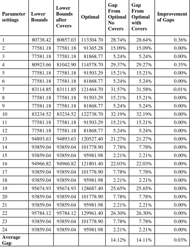
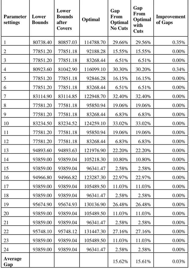
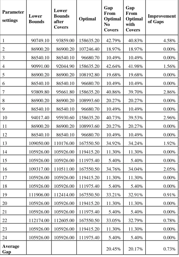
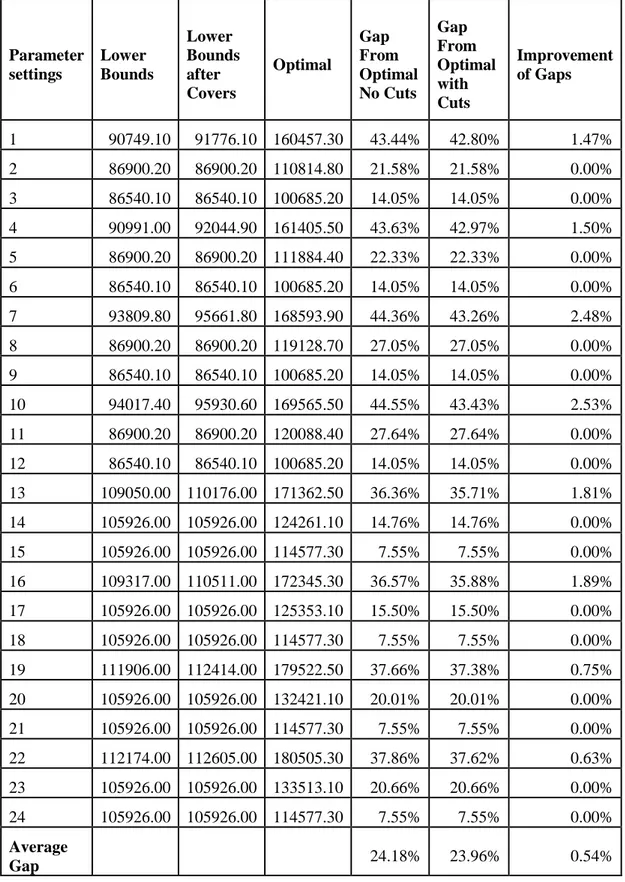
Table 7.1: Heuristic results for Scenario 1 without cover inequalities. ... 54
Table 7.2: Heuristic results for scenario2 without cover inequalities. ... 55
Table 7.3: Heuristic results for scenario3 without cover inequalities. ... 56
Table 7.4: Heuristic results for scenario 4 without cover inequalities. ... 57
Table 7.5: Heuristic results for scenario1 with cover inequalities. ... 58
Table 7.6: Heuristic results for scenario2 with cover inequalities. ... 59
Table 7.7: Heuristic results for scenario3 with cover inequalities. ... 60
Table 7.8: Heuristic results for scenario4 with cover inequalities. ... 61
Table 7.9: Result of heuristic method. ... 62
Table 7.10: Number of solutions with gaps under 1%. ... 63
Table 7.11: Table of random fixations. ... 63
Table 7.12: Results of Scenario 1 with random combinations. ... 64
Table 7.13 : Results of Scenario 2 with random combinations. ... 65
Table 7.14: Results of Scenario 3 with random combinations. ... 66
Table 7.15 : Results of Scenario 4 with random combinations. ... 67
1
1. INTRODUCTION
Considering distribution systems, one of the key factors is the efficient transportation. According to Hoff et al. (2010) in general logistic costs constitute about 20% of the total cost of a product. Logistic costs can be reduced significantly by determining the fleet sizes efficiently since the owning and maintatining a fleet is a major cost componenet in total logistics cost for the firms that keeps a fleet.
Generally speaking, a fleet, is composed of heterogeneous vehicles. In the industry, the vehicle fleets are used for long periods of time, and in these period a fleet will gain different vehicles due to technological developments and market situations. During this period vehicle’s maintenance, operation and depreciation costs will change. Another reason for preferring heterogeneous vehicle fleet is the operational constraints, and also the benefits which this flexibility provides inherently.
The vehicles distinguishing characteristics are divided into three categories:
Physical dimension
Compatibility constraints
Costs
Physical dimensions such as length, height and width of a vehicle determine its carrying capacity. In road based transportations, sometimes physical dimensions obstruct reaching the route networks. As an example for this situation, we can mention the urban areas and narrow roads in villages, and limited space in ramps for loading and unloading. Dimension and weight constraints can vary during a given time horizon, as in seasonal axle pressure limits due to spring thaw. The vehicles speed, can also be categorized under physical dimensions class. Although vehicles with lower speed usually have lower unit cost, it is impossible to give less cost-efficient solutions due to temporal constraints.
2
Except physical dimensions, there exists another characteristic which limits vehicles utilization; “compatibility constraints”. These constraints can sometimes limit the places to which vehicles travel and also the loads which vehicles can carry. Often, customers need vehicles that have special equipment for loading and unloading operations. Operating vehicles in some areas necessitates special certificates. To illustrate this, we can mention the urban areas wherein fuel and noise emissions can limit vehicle utilization.
Another factor which affects vehicle fleet composition is the vehicle costs. Large vehicles usually have lower unit costs in comparison to small vehicles if their capacity is utilized effeciently. As mentioned before, when making decision about fleet compositions for a long period of time, the decision makers first of all have to make a strategic choice between renting and owning the vehicles in their fleet. Comparing the expected costs and incomes under uncertainty is one of the components which should be assessed before deciding about the fleet composition. As it is an important part of the total cost of logistics, the cost related to inventory must also be controlled efficiently. Inventory cost is composed of holding cost, and fixed replenishment cost. In recent years, a business application called “Vendor Managed Inventory (VMI)” is applied by the firms which aim at minimizing the inventory costs. VMI systems are the systems in which the customer’s inventories are totally controlled by the vendor. Vendor decides when and how much to replenish each customer under the limits and constraints that customers determine, e.i. the minimum and maximum inventory level. VMI systems have many benefits on supplier’s side. As long as the supplier does his responsibility of controlling inventory levels and omitting stock outs, supplier can be locked into a VMI system supplier-customer relationship for a long period of time. In this way there will be a steady income for the supplier and the risk of supplier changes on the side of customer will be reduced. In a VMI system, the supplier has the chance of planning his operations more efficiently due to the ability of monitoring customer’s inventory levels in a steady manner. Additionally, during this monitoring procedure the suppliers have a much better understanding of the customer’s consumption rates during a given period of time which will cause decreases in stock amounts. Planning
3
customer’s replenishments actually means that the supplier is determining the orders he faces largely by himself, and thus can make more effective production and replenishment decisions. In addition to all these benefits, a VMI system affords the supplier with the last customer’s demand instead of the filtered demand information provided by the firms and thus can make better demand forecasts.
In supply chains, demand variability increases as moving downwards the chain. In the literature this phenomenon is called “bullwhip effect”. Bullwhip phenomenon occurs due to material and information flows which are not done on the right time and with the right quantity throughout the supply chain. According to Hohmann and Zelewski (2012) another definition of bullwhip effect is the increase in variability of orders as a result of increase in customer demands. As illustrated formerly, in such a situation the flow of information and material along the supply chain layers will not be steadily. When bullwhip effect occurs, the orders look as if they have been hit by a whip and are fluctuated. This fluctuation in orders leads to higher inventory held in the warehouses and also quick responses to customer orders will not be guaranteed anymore. The factors which are effective in appearance of bullwhip effect are generally categorized as five groups: demand distortion, feedback misunderstandings, batch ordering, cost fluctuations and strategic behaviors. VMI systems are able to decrease the bullwhip effect in the supply chains to which they are applied due to their ability of allaying the demand distortion and feedback misunderstandings.
Considering transportation costs, VMI provides several benefits for the suppliers in the cases that customers are highly dispersed through various geographic regions. VMI makes it possible for the suppliers to send customer orders in consolidated form which will cause more efficient utilization of vehicles and as a result declines in transportation costs are met.
On the customer’s side, the most important aspect of VMI application is the decline in inventory holding costs. In many situations the customers make a payment of the amounts which they have sold and are not forced to pay the opportunity type costs. Furthermore, the application of VMI yields elimination of other inventory management related costs such as labor costs, supervisory costs on customer’s side.
4
In this thesis, we tackle a problem of simultaneously determining replenishment plans and fleet sizes. As mentioned in the literature, determining fleet composition needs solving vehicle routing problems. Finding optimal solution to vehicle routing problems requires a set of exact data about the locations of the customers, and leads into long solution times. We did not include exact routing in our modeling, which simplified the model drastically. There are several reasons for this simplification; First, the routing costs constitute relatively small portion of the total cost we have in our model and including routing cost in an aproximate fashion would not change final decisions significantly. Second, our model is a startegic model which considers routing cost in an approximate fashion since the exact routing and its costs would change from day to the next in a real problem. In the strategic type of problems the route length/ cost is assumed to be an approximate value in the literature as we point out in the literature part below. In general, the most of the studies in literature consider operational routing problems and to the best of our knowledge there are some papers which study strategic fleet sizing models. Among these fleet sizing models, none of them considers predetermined delivery frequencies and inventory related costs in a single model, which is the setup of our problem.
As a solution approach to our problem we suggested a “ fix and optimize” heuristic. In this approach the main problem is divided into smaller sub problems. At each iteration, decision variables of one sub problem are defined as integers and the variables for other sub problems are linearly relaxed. After finding a full integer solution through utilization of this pattern, an improvement stage is executed.
This thesis is organized as below: first we will define our problem and analyze the complexity of the problem we have considered. Next the relevant literature is reviewed in chapter 3. After reviewing literature we will present numerical analysis of the problem in chapter 4. In chapter 5, valid inequalitis and lower bound analysis is illustrated. In chapters 6 and 7, we will present the heuristic we suggested and investigate the performance of the suggested heuristic. At the end, we summarize our work and contribution.
5
2. PROBLEM DESCRIPTION AND FORMULATION
In this section we formally state the problem we tackle. Basically, in our problem setup we aim at minimizing sum of the transportation and the inventory cost of shipping a product from one origin to multiple customer destinations. Mainly, by bringing solution to the problem under study, we intend to decide how often and how much to replenish each customer along with the determination of the composition of vehicle fleet. A single product with deterministic demand is made available at the origin and the product is demanded at multiple destinations with a constant rate. A set of heterogeneous vehicles is used to ship the product to the customers. Vehicles vary in different aspects such as carrying capacity, cost per kilometer, and ownership costs. Replenishments are carried out based on a set of given frequencies, which are, in general, on weekly basis. To exemplify, a customer can be replenished weekly, biweekly, thrice or quarto-weekly on any day of the week. Additionally, we can also have a daily frequency. In total, we have 21 different possible frequencies (4*5+1=21).
We are mainly concerned with determining the fleet size and the planning of the deliveries to the customers. To be more precise, the decisions our model will make are the number of each type of vehicle in the fleet of the vendor, along with the frequency, and the vehicle type with which each customer should be served.
Our objective function reflects a total annual cost and it is composed of two different types of costs; transportation related and inventory related costs. Transportation related costs consist of vehicle ownership costs and routing costs. Inventory related costs are fixed replenishment costs at the customers and inventory holding costs. All of these cost components are in the form of annual cost.
We also made some assumption regarding operational issues in our problem. Each customer must be served using a single vehicle and a single frequency. This assumption is in line with practice as customers would prefer regularity of single
6
frequency in delivery. Considering real life situations, daily traffics, and long distances, we assume that each vehicle can make one route in a day and there is a constraint on the number of customers a vehicle can visit on its daily route. We also take into account the fact that customers can be grouped geographically, and two customers from different geographic regions may not be on the same route.
An important aspect of our model is that it does not involve detailed routing decisions. Routing cost is taken into account in an approximate fashion as the product of the number of customers visited in a route and an average cost of travel between customers. The reason for this modeling approximation is that our model is a strategic one integrating several cost factors and routing cost is only one of these factors. Therefore, it is not worth to make the model very complicated to represent only one of the cost components in a detail manner. Besides, the routing cost, in general, does not represent a significant portion in the total cost that we consider in our approach.
In the formulation, we use the notation given below:
Sets:
I : Set of customers V : Set of vehicles
F : Set of frequencies, F= {1, 2, ..., 21}
𝐹𝑗 : Set of coinciding frequencies, ∀𝑗 = 1, … , 𝑛 D : Set of days of the week, D = {1, 2, …, 5} H : Set of weeks per year, H = {1, 2, … , 52}
Parameters:
7 m : Number of customers
𝑟𝑣 : Approximate routing cost between two customers (fixed per kilometer cost of
each vehicle)
g : Dead heading cost
𝑎𝑣 : Annual ownership cost of vehicle type v
𝜆𝑖𝑓 : Annual demand of customer i
h : Annual inventory holding cost per unit of a product 𝑘𝑖𝑓 : Fixed cost of replenishing customer i using frequency f
𝑠𝑚𝑎𝑥: Maximum number of customers that can be visited during the day 𝑐𝑣 : Capacity of vehicle type v
M : A big number
𝑝𝑓 : Total number of annual replenishments for frequency f
𝑡𝑖𝑘 : Incidence matrix of customers i and k (customers i and k can be in the same route if 𝑡𝑖𝑘=2, and cannot be in the same route when 𝑡𝑖𝑘=1)
Using the notations above the mathematical model can be represented as follows:
Min ∑𝑣∈𝑉𝑔𝑝1𝐿𝑣1+∑𝑑∈𝐷∑ℎ∈𝐻∑𝑣∈𝑉𝑔𝑅𝑑𝑣ℎ+∑𝑣∈𝑉∑𝑓∈𝐹𝑟𝑣. 𝑝𝑓. 𝐶𝑣𝑓 + ∑𝑣∈𝑉𝑎𝑣. 𝑉𝑣 +∑𝑖∈𝐼∑𝑣∈𝑉∑𝑓∈𝐹𝜆𝑖𝑓. ℎ. 𝑋𝑖𝑣𝑓. (21) + ∑𝑖∈𝐼∑𝑣∈𝑉∑𝑓∈𝐹𝑘𝑖𝑓𝑋𝑖𝑣𝑓 Subject to: (2.1) ∑𝑖∈𝐼𝑋𝑖𝑣𝑓= 𝐶𝑣𝑓 ∀ 𝑣 ∈ 𝑉, ∀𝑓 ∈ 𝐹 (2.2) ∑𝑣∈𝑉∑𝑓∈𝐹𝑋𝑖𝑣𝑓=1 ∀ 𝑖 ∈ 𝐼 (2.3)
8 𝑀 𝐿𝑣𝑓 ≥ 𝐶𝑣𝑓 𝐿𝑣𝑓 ≤ 𝐶𝑣𝑓 ∀ 𝑣 ∈ 𝑉, 𝑓 ∈ 𝐹 ∀ 𝑣 ∈ 𝑉, 𝑓 ∈ 𝐹 (2.4) 𝑠𝑚𝑎𝑥𝑉𝑣 ≥ ∑ ∑𝑖 𝑓∈𝐹𝑋𝑖𝑣𝑓 ∀ 𝑣 ∈ 𝑉 (2.5) ∑𝑖∈𝐼𝜆𝑖𝑓𝑋𝑖𝑣𝑓≤ 𝑐𝑣 ∀𝑣 ∈ 𝑉, ∀𝑓 ∈ 𝐹 (2.6) ∑𝑖∈𝐼∑𝑓∈𝐹𝑗𝜆𝑖𝑓𝑋𝑖𝑣𝑓 ≤ 𝑐𝑣 ∀ 𝑣 ∈ 𝑉, ∀𝑗 = 1, … , 𝑛 (2.7) ∑ 𝐶𝑣𝑓 𝑓∈𝐹𝑗 ≤ 𝑠𝑚𝑎𝑥 ∀ 𝑣 ∈ 𝑉, ∀𝑗 = 1, … , 𝑛 (2.8) ∑𝑓∈𝐹𝑗𝑋𝑖𝑣𝑓+∑𝑓∈𝐹𝑗𝑋𝑘𝑣𝑓 ≤ 𝑡𝑖𝑘 ∀𝑣 ∈ 𝑉, 𝑖 ∈ 𝐼, 𝑘 ∈ 𝐼, ∀𝑗 = 1, … , 𝑛 (2.9)
Objective of the problem is to minimize the total cost of transportation, inventory holding and replenishment operations. Transportation costs are presented in the form of separate elements such as dead heading costs, routing costs as an approximate value, and ownership cost. Here in our model, dead heading cost is defined as the cost of travelling from vendor to the first customer and from the last customer in a route back to the vendor. Routing costs are integrated to the model as approximate values. Cost of making a route is given by the multiplication of number of customers
𝑅𝑑𝑣ℎ ≥ 𝐿𝑣𝑓-𝐿𝑣1 ∀𝑣∈𝑉, d ∈ 𝐷, f∈𝐹𝑗, h∈H (2.10) 𝑋𝑖𝑣𝑓 ∈ {0,1} ∀ 𝑖 ∈ 𝐼, ∀𝑣 ∈ 𝑉, ∀𝑓 ∈ 𝐹 (2.11) 𝐿𝑣𝑓∈ {0,1} ∀𝑣 ∈ 𝑉, ∀𝑓 ∈ 𝐹 (2.12) 𝐶𝑣𝑓∈ 𝑍≥0 ∀𝑣 ∈ 𝑉, ∀𝑓 ∈ 𝐹 (2.13) 𝑉𝑣 ∈ {0,1} ∀𝑣 ∈ 𝑉 (2.14) 𝑅𝑑𝑣ℎ ∈ {0,1} d ∈ 𝐷,v ∈ 𝑉, h∈H (2.15)
9
which are replenished by vehicle type v and frequency f and an average cost per kilometer of vehicle type v. Annual ownership cost is calculated as the product of number of type v vehicles and the corresponding ownership cost for that type of vehicle. Other two cost components (holding and replenishment costs) are used as it is in well-known EOQ model.
By constraint (2.2) we determine the number of customers being replenished by vehicle type v and frequency f. Demand satisfaction condition is forced by adding constraint (2.3) to the model. With constraint (2.4), we make sure that 𝐿𝑣𝑓 is one if we use any vehicle v and frequency f to cover any customer demand. By utilizing (2.5) we determine if a vehicle is used for replenishing any customers, or not.
It is always important not to overload the vehicles. To meet this restriction, we utilized constraint (2.6). Total amount being shipped to customer i which is replenished by vehicle type v and with frequency f must be less than available capacity of vehicle v. This condition must hold for all of the 21 available frequencies. In our problem, the largest loads are shipped on coinciding frequencies and capacity must not be exceeded, and this restriction is forced by constraint (2.7). Obviously, in real life situations, the number of customers which can be visited on a specific route depends on the distances, traffic and some other factors. We embedded this constraint in our model as constraint (2.8), which forces the routes to consist of customers less than a predetermined maximum number of customers. For tackling geographically dispersed customers we used constraint (2.9) which allows us to take some customers in a route and exclude the ones which are not eligible to enter this specific route. Entrance eligibility is given by the incidence matrix, which has value of 1 representing the customers that are not allowed to be on the same route, and value of 2 for the ones which are eligible to enter the same route. By addition of constraint (2.10) we omit the extra repetition of deadheading cost. To handle this extra cost of redundant dead headings we check if there is any vehicle that replenishes any customer with daily frequency. In the case that such a customer exists, all other frequencies assigned to that specific vehicle will be set to zero and their deadheading cost will not affect the objective function value. Actually, in this constraint we subtract 𝐿𝑣1 from all other 𝐿𝑣𝑓 variables and set 𝑅𝑑𝑣𝐻 as greater or
10
equal to subtraction of these two variables. In this way if for example vehicle 1 replenishes any customer daily, all of the 𝑅𝑑1𝐻 variables become zero and daily trips
number are multiplied with fixed deadheading cost parameter. On the other hand, if no vehicle is assigned to daily frequency, based on the correspondence between f values, d and H (for example f =3 means weekly Tuesdays and corresponds to the second day of the week, that is d = 2 and H = 1,.., 52) the related 𝑅𝑑𝑣𝐻 is equated to 1
and is multiplied by deadheading cost. (2.11)- (2.15) present the domain for the decision variables.
2.1 Problem Complexity Analysis
In this section we show that the problem tackled in this thesis is a NP-Hard problem through polynomial time reduction from the “One- dimensional bin packing problem” which is proved to be strongly NP hard in E. G. Coffman et al. (1997). In the bin packing problem, objects of different volumes must be packed into a finite number of bins or containers each of volume V in a way that minimizes the number of bins used.
Considering our problem, under some assumptions we can transform the current problem to bin packing problem in pseudo-polynomial time. Consider the scenario for our problem where there is a single vehicle type, a single frequency, no clustering, and all the costs excluding the vehicle ownership cost are equal to zero. Also assume that ownership cost fo a vehicle is equal to 1. This setup is equal to following parameter setting for our problem:
F= {1}, n = 𝑟𝑣 = g = 𝑘𝑖𝑓 = h = 0, 𝑠𝑚𝑎𝑥=∞, 𝑡𝑖𝑘=2 for all (i, k) pairs, 𝑎𝑣= 1 for all vehicles.
Under this setting our problmes turns into one dimensional bin packing problem, where we try to minimize the number of vehicles.
11
3. LITRATURE
The problem tackled in this thesis is the problem of replenishment planning along with the fleet size determination. To the best of our knowledge among the researches in the literature, there is not any paper which integrates replenishment and fleet size planning problems. Generally speaking, the researches done on the field of our interest have usually ignored detailed transportation costs which correspond to nearly 60% of total costs in distribution systems. One other aspect which makes our problem different from the researches existing in the literature of subject is the approximate route costs. The works done on routing problems are using vehicle routing solution methods to a great extent which usually causes difficulty in terms of solution times and data gathering. We utilized approximate routing costs in order to simplify the process of problem solution.
Along with all these discrepancies, there are some papers which are close to the problem we considered to some extent. Shipment planning problems which utilize predetermined frequencies, fleet sizing problems, inventory routing problems, the papers which applied fix and optimize heuristic and also the researches about continuous approximation models are among the fields which have some aspects in common with the problem of consideration.
3.1 Predetermined Frequencies
One of the papers which uses predetermined frequencies is Bertazzi et al. (1997). As in our paper, products are shipped from one origin to multiple destinations with a set of given frequencies. Another similarity to our study which makes the mentioned paper interesting for us is the objective of the problem, which is to minimize the costs occurring during transportation and also inventory related costs. Here the approach for solving the problem consists of two phases. First they apply a heuristic based on solving the model as a single link problem. The second phase is dedicated to local improvement of the solution achieved in the previous step. In Bertazzi and
12
Speranza (2002), the problem of shipping several products from a common origin to a common destination is considered. The objective function of the problem aims at minimizing the sum of inventory and transportation costs as it is in our problem. There are two cases considered in Bertazzi and Speranza (2002): deriving a shipping strategy in existence of continuous frequencies and a set of given discrete frequencies. In this work transportations costs are not considered in detail. That is, dead heading costs and vehicle ownership costs are not integrated to the model. These cost factors constitute a significant part of distribution systems’ total costs. Another important point which is neglected in the studies existing in the litrature is that generally routing costs are not considered. Another outsanding charactristic of our problem which makes it significant is that all the inventory related costs, i.e. holding cost, replenishment costs are considered in our model.
Another work considering feasible predetermined frequencies is Maria Grazia Speranza and Ukovich (1994). In this work, integer and mixed integer linear programming models are developed for four situations. Assumptions of the problem tackled in this study are the proportionality of transportation costs with the number of journeys that a typical vehicle makes, and the demand divisibility. Luca Bertazzi (2000) considers the problem of shipping several products from an origin to a single destination under a predetermined frequency set. In this paper dominance rules are derived and the efficiency of a branch and bound algorithm is improved using these dominancy rules. Additionally, some heuristics are suggested and compared with EOQ-type algorithms. Bertazzi and Grazia Speranza (1999) investigates the problem of minimizing sum of the inventory and transportation costs in the multi-products logistics with one origin, some intermediate nodes, and a destination in existence of predetermined frequency set. As a solution approach heuristics based on decomposition of sequences or based on the solution of simpler problems are proposed. One other research work done by Bertazzi et al. (2005), which also has some aspects in common with the subject under consideration in this paper, tackles a complicated production-distribution system in which several items are produced repeatedly, and they are distributed to a set of retailers using a fleet of vehicles. VMI strategy studied in their work is evaluated in two categories and two different decompositions of the problem along with presented optimal or heuristic procedures
13
for the solution of the sub problems. In M. G. Speranza and Ukovich (1996) again the problem of distributing various products from a single source to a multiple set of destinations in existence of the given frequencies is studied. Here, the Np-hardness of the problem is proved and a branch and bound method is applied as a solution method.
In general, in works which have considered predetermined frequencies the replenishment costs are not taken into consideration. Additionally, ownership costs are ignored and are not included in the mathematical models which they suggested. Another difference of our model from these works is that we consider routing costs in two different parts, i.e. deadheading and cost of travelling between two customers, while in predetermined frequency works transportation costs are taken as a value proportional to number of trips that a vehicle makes. In our model, we consider coinciding frequency effects which is neglected in the works mentioned above. To summarize, our problem is more detailed and includes all the costs which can effect the replenishment and fleet sizing decisions.
3.2 Fleet Sizing Problems
In Baldacci et al. (2008) an overview of approaches for solving heterogenous VRPs is given and as no exact algorithms has been presented for the problem under consideration, some lower bound assessments are given. In Żak et al. (2011) a fleet sizing problem in a road freight transportation company with heterogeneous fleet is considered. Sayarshad and Ghoseiri (2009) suggested a new formulation and solution procedure for optimizing the fleet size and freight car allocation wherein as in our problem car demands are assumed to be deterministic. Crainic (2000) introduces a new classification of service network design problems and formulations in addition to presentation of a state-of-the-art review about studies on service network design modelling and mathematical formulation developments for network design. Another research paper which deals with a problem that has some aspects seeming similar to the problem we have focused on in here, is the work done by Desrochers and Verhoog (1991). In their paper, a problem of simaltaneously selected composition and routing of a fleet of vehicle is addressed wherein customer demands are known and are from a centeral depot. As a solution approach, a new savings heuristic is
14
used. One of the aspects which makes our problem different from their work is that we utilize a strategic routing problem. To illustrate, fleet sizing problems in general use exact routing algorithms which requires large amounts of precise data and excessive solution times. Conversely, in our research we use average cost of the leg between two customers as an approximate value which will simplify the problem solution to a large extent considering the slight effect that routing cost has in total transportation costs.
3.3 Inventory Routing Problems
The inventory routing problem is a problem in which inventory management, vehicle routing and delivery schedualing decisions are made simaltaneously. Generallay, in these class of optimization problems, a single product is shipped from a single origin to multiple destinations in a period of T while total cost of all operations is minimized. The demand for a typical customer i is equal to 𝑢𝑖 and each customer is able to keep a local inventory of product up to a maxmimum of 𝐶𝑖. Customer i has the inventory equal to 𝐼𝑖 at time 0. For accomplishing shipments a homogeneous fleet
of m vehicles is available. Carrying capacity of each vehicle which is included in the available fleet is equal to Q. Here the objective is to minimize the distribution costs and also obstruct stockouts at any of the customers.
According to Campbell et al. (1998) in a typical inventory routing problem we are about to make three important decisions as below:
When to serve a customer?
How much to deliver to a customer when it is served?
Which delivery routes to use?
One of the papers which we analyzed under the category of IRP( Inventory Routing Problem), is Leandro C. Coelho (2014). In this research inventory routing problem is defined as a combination of vehicle routing and inventory management problems in which a supplier has to deliver products to a number of geographically dispersed customers, subject to side constraints. The paper aims at reviewing the IRPs with respect to their structural variants and the availability of information in customer demand. Coelho and Laporte (2013) has proposed a branch and cut algorithm for the
15
exact solution of several categories of inventory routing problems. Another review paper is the one by Moin and Salhi (2007) which classifies the models of IRP based on the planning horizon they have employed. The aspect which makes IRPs similar to problem of our interest is that in both problems demands of geographically dispersed customers are distributed.
The most important differences of our problem from IRPs are the main focuses of our problem, which are determining the composition of the fleet considering the ownership cost, and the assignment of both frequency and vehicles to customers considering detailed inventory related costs. In terms of delivery frequencies, as mention in problem definition section, we utilize predetermined frequencies which, to the best of our knowledge, is not generally utilized in inventory routing problems. Inventory routing problems are extensions of vehicle routing problems and are classified as operational problems. Here, we do not attack an operational problem, instead we suggest an strategic problem which uses approximate routing costs instead of solving vehicle routing problems.
3.4 Fix And Optimize Heuristic
In order to understand the heuristic method which we decided to apply to our model in this thesis research comprehensively we investigated the papers which applied this approach to various problems previously. One of the researches is Gintner et al. (2005) in which fix and optimize heuristic is used for bus scheduling problem. Federgruen et al. (2007) has applied the fix and optimize heuristic to multi-products, capacitated lot sizing problem. In Helber and Sahling (2010) the same heuristic is utilized for soling the multi-level capacitated lot sizing problem. One problem which has some similarities to our problem is the one studied in Dorneles et al. (2014). The problem considered in this research is a full integer problem with all variables defined as binaries except for one integer variable. Fix and optimize heuristic is applied to the problem and the efficiency of the algorithm is analyzed. It is stated that the proposed fix and optimize heuristic were able to find new best known solutions for seven instances including three optimal ones.
16
3.5 Continuous Approximation Models
As mentioned before, here we consider a strategic problem, thus the routing costs are taken as approximated values. Jabali et al. (2012) presents a cotinuous approximation model for determining the long-term vehicle fleet composition needed for performing distribution activities. As in our problem, vehicles differ in terms of their capacities, fixed cost per kilometer and an extra difference which is route durations. The assumption here is that customers are dispersed in a circular service region which is partitioned into zones that each of them are serviced by a single vehicle. The routing costs are assessed by means of a continous approximation model as we will do in our research. Huang et al. (2013) also uses continuous approximation model for routing teams to different communities to assess damage and relief needs following a disaster. The model named as continuous approximation model yields solutions which are easily implemented and reduces the neccassity for detailed data and computational requirements. In our problem we use the routing cost of a leg between two customers as an approximate value. As mentioned before, in total, routing costs constitute a small portion of costs of distribution systems in comparison with total cost of a product. As a result, handling the routing costs as approximate values will not affect the decisions which are to be made in a great extent inspite the simplification it causes in problem solution. In the problem which we have worked on, we calculate the routing costs as multiplication of an approximate route cost, number of customers being replenished with a specific vehicle type and a specific frequency and total number of replenishments per year.
17
4. NUMERICAL ANALYSIS OF THE PROBLEM
The problem tackled here, is an integration of fleet sizing and replenishment planning problem and it is presented as a mixed integer programming model. Several customers must be replenished by a single frequency and a single vehicle. In order to have an understanding of the behavior of the solution of our problem and derive some managerial insight, we have solved the model under four different demand scenarios, and 24 different parameter settings. We used CPLEX OPL V. 12.4 on a PC with Intel Core i7-3612QM 2.10 GHz processor, 6.00GB of RAM. Solution time for all of the scenarios was under 2 hours except for the parameter settings which were not solved to the optimal in 2 hours. The problems solved optimally took a time period from a few minutes to more than half hour.
In this section, we will first introduce the data set we utilized, then we will explain the scenarios and parameter settings. Finally will present analysis based on the results we obtained.
4.1 Data Set
We worked on a problem composed of 20 customers with deterministic demand. The annual demand values are sampled randomly from a uniform distribution between 80 and 120 (𝐷𝑖 ∈ Uniform [80,120]). The demand is presented on annual basis
considering the possible frequencies. We have a given set of discrete frequencies, which are daily, weekly, biweekly, thrice-weekly, and quarto-weekly. Thus, we have 21 different frequencies available (5*4+1). As mentioned previously, demand has been adjusted considering available frequencies, that is, the annual demand for a customer being replenished every week is calculated as “annual demand/number of weeks in a year “, etc. Another cost parameter to be considered is the cost of replenishment operations presented by “k”. k is also adjusted according to the available set of frequencies, that is, the k value for a customer being replenished biweekly is calculated as “k *(number of weeks in a year/2)”. Here k is equated to
18
50. Since replenishment costs are calculated as multiplication of k, annual replenishment number and the customer demands, number of possible replenishment in one year must be applied to the model. For this purpose, we defined parameter 𝑝𝑓 which represents the number of replenishments during one year under frequency f. To illustrate more, suppose one customer is replenished thrice-weekly. The number of replenishments occurring during a year of thrice-weekly replenishments is calculated as: P(f) = 52/3 (It is obvious that we have 52 weeks in a year). Holding costs usually play an important role in making replenishment decisions. Sometimes extremely high holding cost factors force the decision maker to choose more frequent replenishment plans in order to trade-off the replenishment and holding costs. Conversely, a system with very low holding costs will prefer less frequent replenishments to save more of transportation and replenishment costs. Thus, holding cost is an important factor, here in our study, we used a holding cost of 300 and 600 for different scenarios.
For accomplishing transportation operations, we have unlimited number of heterogeneous vehicles. Mainly, the vehicles differ in carrying capacity, ownership cost and costs per kilometer. In terms of carrying capacity, we have three types of vehicles in hand. Capacity of these vehicles is calculated based on weekly, bi-weekly and thrice-weekly demands of customers. Average annual demand of customers is equal to 100. On average, the daily demand of a customer is about 0.27397 (100/365). Calculating the same customer’s weekly demand we have “number of days in a week * daily demand” which is equal to: 5*0.27397=1.36986. As mentioned before, we have a constraint on the maximum number of customers which a vehicle can visit on a single day. Each vehicle can at most visit 5 customers during a single day and thus the lot size which it carries is equal to 5*1.36986= 6.85~7. Thus, the smaller vehicle’s carrying capacity is set to 7 units. The same procedure was applied to the vehicles with carrying capacity based on bi-weekly and thrice-weekly replenishment plans and the result was 14 and 21 units. Carrying capacity for the larger vehicles is calculated as “smaller capacity+40%*smaller capacity” which equates to 10 units for smaller vehicles with capacity 7, to 20 for smaller vehicles with capacity 14 and to 27 for smaller vehicles with capacity 21.
19
Ownership costs include all the vehicle related costs such as depreciation costs, labor costs, taxes and etc. The ownership cost for smaller capacities is equal to 40800 TL/year. Ownership costs were adopted from Ertogral and Gonzalez (2015), and reflect real life situation costs. For the case in which larger carrying capacities are considered, two situations are tackled. One of this situations is the one in which the vehicle with larger capacity cost the vendor “40800+ 20%*40800” and the other situation is which the vendor faces the cost equal to “40800+ 40%*40800”.
In addition to ownership costs, cost per kilometer factor affects the total expenses. In general, among the papers existing in the literature of inventory routing and distribution systems, routings is done based on solving normal VRP or IRPs. Bringing optimal or near optimal solutions to routing problems needs accurate data and also a plentiful amount of solution times. This aspect of routing problems makes them difficult for handling in everyday life. Here in this thesis, we used cost per kilometers as approximate values which will simplify the process of solving the problem. Cost per kilometer of vehicles, 𝑟𝑣, with smaller carrying capacity is equated
to 7 which was adopted from the research done by Ertogral and Gonzalez (2015). Cost per kilometer of vehicles with higher carrying capacity is calculated as “cost per kilometer of smaller vehicles + 20% *cost per kilometer of smaller vehicles” and “cost per kilometer of smaller vehicles + 40% *cost per kilometer of smaller vehicles “.
In some real life situations we face the customers that are dispersed widely in very distant geographical locations. Putting all these customers together on the same route will not be possible all the time. To handle such circumstances, we defined an incidence matrix which represents the fact that customer i cannot be on the same route with customer k or vice versa. Elements of incidence matrix are expressed as value of 1, standing for the customers which are not possible to be visited on the same routes, and 2 for the ones who are free to be on the same routes.
In order to evaluate the results under various scenarios we made use of the incidence matrix in which the customers with the possibility of allocation to the same routes are shown with number 2, and the customers which cannot be on the same route are presented by 1. One other parameter used in the model, is H which stands for the
20
frequencies on the basis of weeks and it is used for deletion of the redundant repetitions occurring on the coinciding frequencies. To illustrate more, H for weekly replenished customers is presented as 1,2,3,…,52 whereas in case of customers being replenished thrice-weekly have H values of 3,9,..,52.
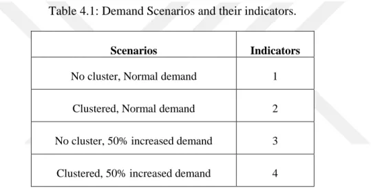
Scenarios being considered here are the problems with normal demand and no/four clusters, and with 50% higher demand no/ four clusters. In each of these four scenarios, effects of each factor (holding cost, cost per kilometer, capacities and…) are investigated and also the changes appeared in costs in cases of the various scenarios are analyzed. The scenarios and parameter settings are as shown below in Table 4.1 and Table 4.2.
Table 4.1: Demand Scenarios and their indicators.
Scenarios Indicators
No cluster, Normal demand 1 Clustered, Normal demand 2 No cluster, 50% increased demand 3 Clustered, 50% increased demand 4
21
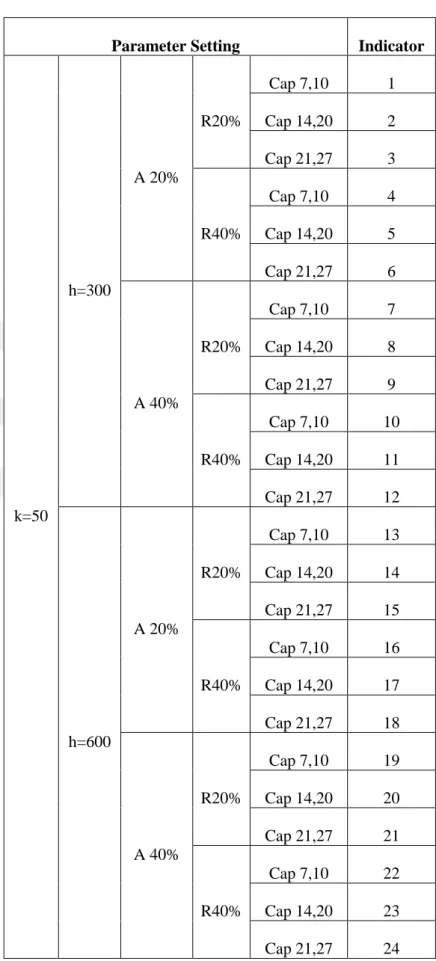
Table 4.2: Parameter settings and indicators.
Parameter Setting Indicator
k=50 h=300 A 20% R20% Cap 7,10 1 Cap 14,20 2 Cap 21,27 3 R40% Cap 7,10 4 Cap 14,20 5 Cap 21,27 6 A 40% R20% Cap 7,10 7 Cap 14,20 8 Cap 21,27 9 R40% Cap 7,10 10 Cap 14,20 11 Cap 21,27 12 h=600 A 20% R20% Cap 7,10 13 Cap 14,20 14 Cap 21,27 15 R40% Cap 7,10 16 Cap 14,20 17 Cap 21,27 18 A 40% R20% Cap 7,10 19 Cap 14,20 20 Cap 21,27 21 R40% Cap 7,10 22 Cap 14,20 23 Cap 21,27 24
22
4.2 Results And Analysis
In this section, we would like to investigate the way that clustering and increase in demand affect the results we get from the problem. In Chart 4.1 we represent the changes in the objective function value in percentages in comparison to base case of each scenario (no cluster, normal demand case is assumed as base for normal demand scenarios, and high demand no cluster is the basis for other two cases).
Chart 4.1: Percentage changes of objective function values.
As it is obvious from the chart, the addition of clusters and increase in demand result in an increase in the objective function value. This increase is sharper for the problems with vehicle capacities of (7,10). This may be due to the capacity limitation which will lead to higher routing costs or replenishment costs. Lower capacities limit the size of the lots which are transported and this will necessitate more frequent replenishments. One of the important parts of objective function is routing cost. In our model, routing cost consists of dead heading costs and travel costs between customers. 0 5 10 15 20 25 30 35 40 45 without clusters,D 4clusters,D without clusters,D50% 4clusters,D50% Objective Values cap7,10 cap14,20 cap21,27
23
Chart 4.2: Percentage changes of routing costs
Routing costs decrease proportional to increase in carrying capacity. The reason is that the lot consolidation possibility is proportional to vehicle capacity. The higher vehicle capacities facilitate more lot consolidation. As it is revealed in the chart, in scenario 4 routing costs increases when the vehicle capacity increases from 14 and 20 to 21 and 27. This increase is due to the utilization of smaller vehicles instead of a combination of large and small vehicles. This change of vehicle utilization may cause the number of replenishments to increase which results in higher deadheading costs. Another situation in which routing costs escalate is demand increase. The reason is that satisfying increased demands with the same vehicle capacity yields utilization of more vehicles which imposes the extra ownership costs to routing cost. Ownership costs also reveal changes along different scenarios.
0 2000 4000 6000 8000 10000 12000 14000 16000 18000 Routing Cost cap7,10 cap14,20 cap21,27
24
Chart 4.3: Percentage changes of ownership costs
The addition of clusters, does not affect the utilization of vehicles with capacities 27 and 21 units. Identically, demand increase does not change the number of vehicles which have capacities equal to 21 and 27 units. That is, the same number of vehicles with capacity 21 is used along all of the scenarios. This may be due to the relation of capacity and lot sizes. The capacity of 21 units is satisfactory amount for handling replenishment of customers with these demand values.
The ownership cost for vehicles with capacities of 7 and 10 increases when customers are divided into clusters and demand is increased. This increase in ownership costs is due to low possibility of lot consolidation in clustered case which leads to utilization of higher number of vehicles. In addition to clustering, increase in demand causes the lot sizes to become larger and it forces the usage of more vehicles to compensate the disadvantage of low capacity. The ownership cost for vehicles with capacities 14 and 20 increases by clustering the customers. The reason for this increase is that optimization tries to reduce the replenishment cost and also routing cost by means of using maximum possible capacity that allows lot consolidation. Ownership cost for the scenario with increased demand and clusters is less than the cost for normal demand and clustered case. The reason for this situation can be explained in terms of vehicle type utilization. In the case with clusters vehicle capacity is used in a way that affords maximum consolidation thus a combination of
0 10 20 30 40 50 60 70 80 90 without clusters,D 4clusters,D without clusters,D50% 4clusters,D50% Ownership Costs cap7,10 cap14,20 cap21,27
25
high and low capacities are used. Conversely, in the case with increased demand and no clusters, consolidation is allowed and no restrictions exist except the vehicle capacity. Thus, there must be a trade-off between ownership and replenishments costs. This tradeoff leads into using low capacity vehicles.
The reason for low capacity utilization is that they have enough capacity which means that the difference between 20 and 14 units of capacities does not worth paying the difference in the ownership costs. Thus here the low capacities are preferred which reduce the ownership cost in comparison to the scenario 1.
Chart 4.4: Percentage change of holding costs
Holding cost in clustered normal demand scenario decreases for all of the capacities because there is a restriction of lot consolidation resulting from routing rule. Routing rules forces some customers not to be on the same route with some other customers. This means that simply a vehicle cannot consolidate the demand of different customers on the same trip. Another restriction for consolidation is the capacity of the vehicles which do not allow the vendor to send lots larger than a specific size. Smaller lots lead to less holding costs.
Holding costs for vehicles with capacities 7, 10 and 14, 20 increases with the demand increase which may be due to the increase in vehicle utilization. That is, in the
-10 0 10 20 30 40 50 60 without clusters,D 4clusters,D without clusters,D50% 4clusters,D50% Holding Cost cap7,10 cap14,20 cap21,27
26
scenario with normal demand and four clusters, total number of vehicles used is equal to 8 while in other scenarios total vehicle number changes to 16 for capacities 7, 10 and 9 for capacities 14, 20.
For the increased demand with clusters the number of vehicles is the same as number of the vehicles in no cluster increased demand case but the combination differs. In this scenario more large vehicle is used which means that much larger lots can be transported. This will lead to higher stocks in warehouses and respectively higher holding costs.
The holding cost value for vehicles with capacities 21 and 27 decreases when customers are divided to clusters and have increased demands. In this case there exists enough capacity for possible consolidation but routing rules will not allow consolidation more than a limited value. Thus the vehicles are transporting lots with lower sizes which cause lower holding costs.
Another cost factor which is affected by the addition of clusters is the replenishment cost.
27
Chart 4.5: Percentage changes of replenishment costs
When clusters are considered in normal demand scenarios, the size of transported lots decreases due to routing rules and thus more frequent replenishments are needed which lead in to higher replenishment costs.
The same pattern is followed by vehicles with capacities 14, 20 and 21, 27 through scenarios 3 and 4. In scenario 4 the replenishment cost for vehicles with capacities 7, 10 decreases. The reason is that an equal number of high and low capacity vehicles are used that have enough capacity for consolidating the amount allowed by routing rules. -10 0 10 20 30 40 50 60 70 without clusters,D 4clusters,D without clusters,D50% 4clusters,D50% Replenishment Cost cap7,10 cap14,20 cap21,27
28
Chart 4.6: Percentage changes of average frequency
Here in this chart, average frequency is calculated as [ (∑ 𝑥𝑖𝑣𝑓∗ P(f) )/ number of customers] and the frequencies are numbers like 1.2 (meaning replenishments are done weekly or biweekly), 2.4 (replenishments are done biweekly or thrice weekly). Our expectation about the decrease in frequencies and more frequent replenishments is met in normal demanded scenarios. These decreased frequencies are due to the addition of clusters and decreased consolidation possibility. In the high demand scenarios addition of clusters results is less frequent replenishments. The reason for frequency increase is that by increasing the time between two successive replenishments we have better consolidated oreders. Higher consolidation causes decrease in replenishment costs while increasing the holding cost.
Lot sizes changes is parallel to the changes occurred in average frequencies. In scenarios with normal demand and clusters, both frequency and lot sizes decrease. On the other hand, in the high demand scenarios, higher frequencies cause lot sizes to grow larger. In this case lot sizes increase for capacities equal to 7-10 and 14-20. The reason is that the demand is increased without changing the carrying capacity. Aditionally, in the scenarios with higher demands for the mentioned capacities(7-10, 14-20) the combination of low and high capacity vehicle utilization is different from the scenarios with low demands, i.e, in general higher number of vehicles are utilized and a shift from high capacity utilization to low capacity utilization is observed.
-35 -30 -25 -20 -15 -10 -5 0 5 without clusters,D 4clusters,D without clusters,D50% 4clusters,D50% Average Frequency cap7,10 cap14,20 cap21,27
29
Conversely, for the vehicles with capacities 21-27 with demand increase lot sizes decrease. This change is due to more frequent replenishments which leads to smaller lot transportation.The percentage changes are shown in Chart 4.7.
Chart 4.7: Percentage changes of average lot
After analyzing the changes in average lot size, the changes in number of vehicles used in each case should be considered. Generally speaking, the addition of clusters in both cases ( high and normal capacities) causes a shif to the large vehicle usage. This happens in order to create a flexibility for demand consolidation. As discussed previously, adding clusters causes less frequent replenishments and larger lot sizes. In order to consolidate demands into these large lot sizes and also for neutralizing the clustering restrictions vehicle selection shifts to large vehicles. The changes are represented in Chart 4.8. -10 0 10 20 30 40 50 60 without clusters,D 4clusters,D without clusters,D50% 4clusters,D50% Average Lot cap7,10 cap14,20 cap21,27
30
Chart 4.8: Number of vehicles used under each scenario
For problems with vehicle capacities equal to 7 and 10 units, in the first two scenarios using larger capacity vehicles (10 unit) is preferred. This may be for reducing the replenishment costs and also the part of routing costs which is proportional to the repetitions in a year. Demand increase leads to utilization of small capacity vehicles. This will increase the average lots and thus holding costs will go higher. In the case of increased demand the reason for small capacity selection can be the limitation that routing rules create. Using larger number of low capacity vehicles allows to consolidate the lots as much as possible while the routing and ownership costs does not increase as much as they would if we utilized high capacities.
Considering the vehicles with capacities 14 and 20, we see that in scenarios 1 and 3 vehicles with capacity of 14 units are used. This capacity maybe enough for consolidating the lots to a desirable level. In scenario 4, larger demands and low consolidation possibilities lead to utilization of more vehicles of capacity 20 which will consolidate more lots if possible.
In case of capacities 21 and 27, the obvious point is that the capacity of 21 units is clearly enough to handle distribution plans and the lot transportation as capacity 27 is never used in any scenarios.
0 5 10 15 20 25 30 35 1 2 3 4 Number of Vehicles cap27 cap21 cap20 cap14 cap10 cap7
31
routes. The reason of this decrease is obviously more consolidated transportation under clustered demand. The changes in route numbers are parallel with our expectations as shown in Chart 4.9.
Chart 4.9: Percentage changes in number of routes under scenarios -40 -20 0 20 40 60 80 100 120 140 without clusters,D 4clusters,D without clusters,D50% 4clusters,D50% Number of Routes cap7,10 cap14,20 cap21,27
33
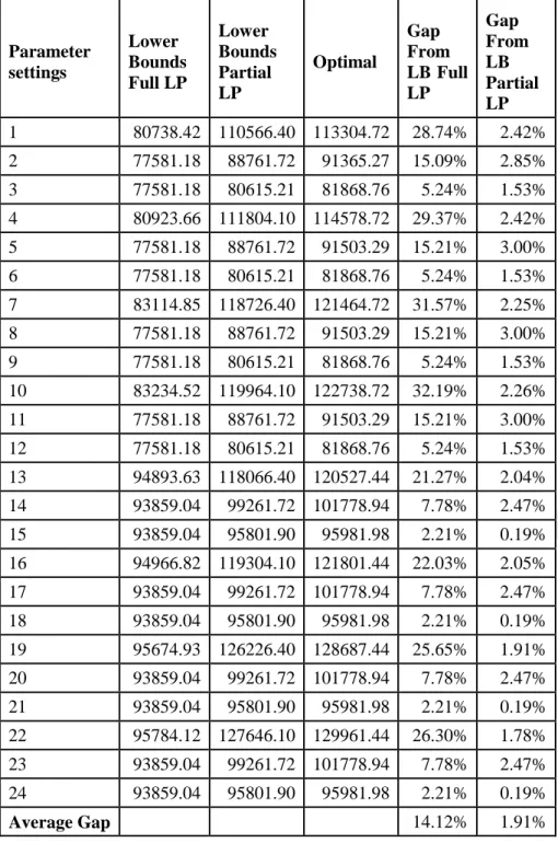
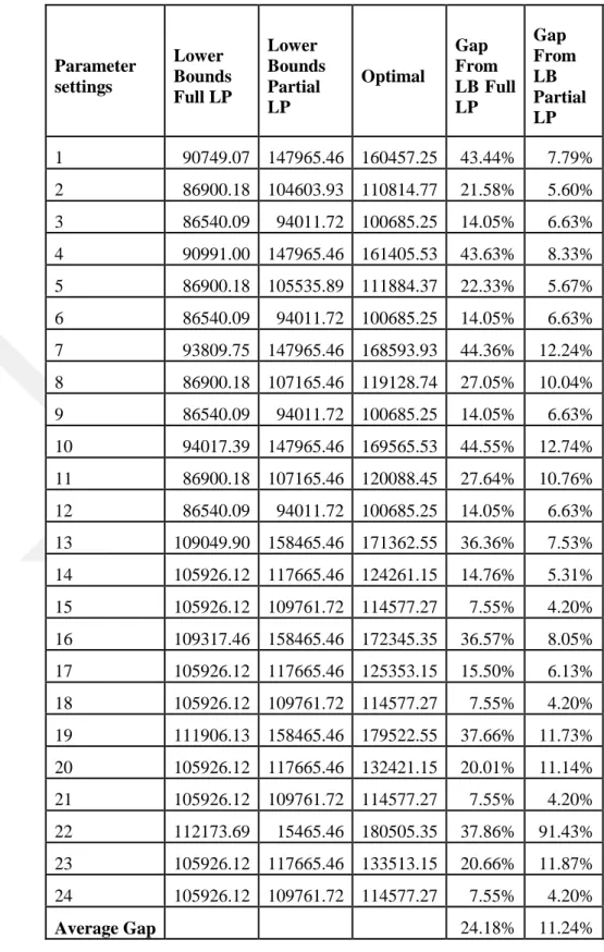
5. VALID INEQUALITIES AND LOWER BOUND ANALYSIS
5.1 LP Based Lower Bound Analysis
As mentioned previously, special case of the problem studied in this thesis can be shown to be a “Bin Packing Problem”, which is known to be Np-hard. This characteristic leads into excessive computational time as the problem size gets larger. For large problems, the performance of our heuristic methods applied to the problem should be compared with the lower bounds of the problems under consideration. The problem considered in this thesis is in form of an integer programming model and all of the decision variables are binaries or integers. We used two types of relaxations for obtaining lower bounds. First method we used is full LP relaxation, in which all of the binary variables are relaxed in the interval [0, 1] and integer variables are taken as belonging to 𝑅+. For further analysis of bounds we
investigated the bounds from partial LP relaxation problems. In this case, all the binary variables except 𝑉𝑣 are relaxed in [0, 1] interval and 𝑉𝑣 is still defined as a binary variable. The integer variable 𝐶𝑣𝑓 is set to be in 𝑅+ . As expected, the results
with a binary variable and other variables as continuous values show a tighter lower bound for the scenarios under study. Problems were solved with commercial solver CPLEX 12.4. Results for different scenarios and parameter settings are given in tables Table 5.1throughTable 5.4.