Turkish Households Consumption Behavior and Flexible Engel Curves

(1)

Doğuş Üniversitesi Dergisi, 18 (2) 2017, 35-50

(1)_{Gümüşhane Üniversitesi, İktisat Bölümü, [email protected]} (2)_{Karadeniz Teknik Üniversitesi, İktisat Bölümü, [email protected];}

Geliş/Received: 14-12-2016, Kabul/Accepted: 16-10-2017

Turkish Households Consumption Behavior and Flexible Engel

Curves

1

Türkiye’de Hanehalkı Tüketim Davranışları ve Esnek Engel Eğrileri Egemen İPEK(1) _,_{Haydar AKYAZI}(2)

ABSTRACT: The aim of this study is to first determine the relationship between

the social and economic differences of households and the functional form of their consumption and then test their consumption behavior empirically. To do so, this paper utilizes the empirical framework of “Exact Affine Stone Index” (EASI), which is offered in Lewbel and Pendakur (2009), by using the Household Budget Surveydata provided by Turkey Statistical Institute, for the 2003-2011 period. The analysis presented here estimates Engel curves, income and demand elasticities for eleven main consumption bundles of the reference household using the Iterative Three Stage Least Squares (I3SLS) method. Differently to previous studies, the empirical results show that the Engel curves have fifth degree polynomial functional form for all consumption groups, except for hotel expenditures for Turkish households. Moreover, this study is capable of measuring the impacts of changes in taste and preferences of Turkish households on their consumption expenditures over the years.

Keywords: Household Consumption Behavior, Engel Curves, Demographics

Variables, EASI, I3SLS

JEL Classifications: D12, D120, C3

Öz

:

Bu çalışmada, hanehalkları arasında mevcut olan sosyal ve ekonomik

farklılıklar ile tüketim arasındaki fonksiyonel yapı tespit edilerek, tüketim davranışlarının ampirik olarak incelenmesi amaçlanmıştır. Bu amaçla, Lewbel ve Pendakur (2009) çalışmasında önerilen “Tam Belirlenmiş İlgin Dönüşümlü Stone İndeksi” (EASI) çerçevesinde ampirik model oluşturularak 2003-2011 dönemi için Türkiye İstatistik Kurumu (TÜİK) tarafından hanehalklarına uygulanan Hanehalkı Bütçe Anketi (HBA) üzerinden tahminlerde bulunulmuştur. İteratif Üç Aşamalı En Küçük Kareler (I3AEKK) tahmin yöntemi uygulanarak, 11 temel harcama grubu için referans hanehalkına ait Engel Eğrileri ile gelir ve talep esneklikleri tahmin edilmiştir. Elde edilen ampirik bulgulara göre, Türkiye için yapılan daha önceki çalışmaların aksine, otel harcamaları hariç diğer bütün mal grupları için tahmin edilen Engel eğrilerinin 5. dereceden polinomal bir yapıya sahip olduğu tespit edilmiştir. Ayrıca bu çalışmada, hanehalkları arasındaki gözlemlenebilen ve gözlemlenemeyen heterojenlik ile yıllar arasında ortaya çıkabilecek zevk ve tercihlerdeki değişimin de tüketim harcamaları üzerindeki etkisi ölçülmüştür.

Anahtar Sözcükler: Hanehalkı Tüketim Davranışları, Engel Eğrileri, Demografik

Değişkenler, EASI, I3

1_{Thispaper is based on İpek (2014) PhD study titled “Demand Systems Theories for}

(2)

36 Egemen İPEK, Haydar AKYAZI

1. Introduction

Understanding of household expenditure behaviors is important for both the policy maker and economic dynamics. The relationship between household income and the quantity of purchase is interpreted by Engel curves in microeconomic theory. Beside income, social and demographic characteristics of household areimportant factors that impact the Engel curves of households.(Howe 1977, Polak and Wales 1981, Blundell at al. 2003)

The significant effect of heterogeneity among households on consumption behavior is caused by observable and unobservable factors. In this respect, the observed effects obtained by the questionnaire forms and the unobservable effects which are not obtained by the questionnaire forms but which have a significant effect on the difference between the households have recently become importance both theoretically and empirically. In the study, it was aimed to estimate the effect of observable and unobservable differences among households on consumption behaviors, as well as to predict the Engel curves without any polynomial constraints. The rest of the paper is organized as follows. Section 2 presents the literature review. Section 3 summarizes datasets and provides descriptive statistics. Section 4 describes the methodology. Section 5 reports the empirical findings. Finally, section 5 presents the conclusion.

2. Literature

The literature related to Engel curves is generally based on linear or quadratic demand system models such asthe Almost Ideal Demand System (AIDS) and variations of this model. However these classic parametric demand models are not be able to involve variety of shapes andare registered by Gorman (1981) rank conditions.

In recent literature, many studies emphasize the importance of allowing the unobserved preference heterogeneityin demand systems. However in many empirical consumer demand models, error terms cannot be illustrated asrandom utility parameters symbolizing the unobserved heterogeneity (Lewbel and Pendakur, 2009:827).To address the issues above, Lewbel and Pendakur (2009) developed a new approach to estimate and explain of consumer demands. They introduced the Stone log price index (Stone, 1954) to model the Exact Affine Stone Index (EASI) class of cost function which haslog real expenditure equal to an affined convert to Stone index exhausted log nominal expenditure. In addition, EASI demand system has an advantage of permission for flexible interactions between curves. It also permits error terms in the model represent to unobserved preference heterogeneity random utility parameters.

The main concentration of demand systems researches in Turkey is food expenditure. Although there are bunch of empirical works show that the structure of food expenditure (Koc and Yurdakul 1995; Sengul and Tuncer 2005, Fidan and Klarsa 2005; Akbay et al. 2007, Akbay 2005; Özer 2003;Bilgiç 2013;Günden et al. 2011; Tekgüç 2012)there is still literature gap on demand system models including all expenditure categories for Turkish households(Nisancı 1998, 2003;Koç and Alpay 2002; Selim 2000; Özçelik and Şahinli 2009;Şahinli 2010;Sengul and Sigeze 2013). Additionally many of these studies are lack of the prices and numerous

(3)

Turkish Households Consumption Behavior and Flexible Engel Curves 37

demographic characteristics that may affect on Engel curve of a Turkish household (Fisunoglu and Sengul 2011; Sengul and Sigeze 2013). In addition, there is no empirical study for Turkey to measure unobserved preference heterogeneity and the effect of time variables in the model to clarify potential quite variation of some characteristics with changing time.

The main motivation of this study is to offer some evidence such as those mentioned above.In this paper, EASI class of cost function model (Lewbel and Pendakur, 2009) is applied to determine consumer demandsof Turkish households under the assumption of local concavity by using the Household Budget Surveys data conducted by the Turkish Statistical Institute for the period of 2003 and 2011.We obtain Turkish case that rejects both quadratic and linear demand specifications in favor of those with higher-order terms in total expenditure. The consumer demands and household budget shares are affected by diversity of demographic characteristicsand time.

3. Datasets and descriptive statistics

Engel Curve and Demand Systems are examined by using the Household Budget Surveys (HBS) data set conducted by the Turkish Statistical Institute (TurkStat) for the years 2003 to2011. In the survey, households were replaced on a monthly basis with households bearing similar characteristics. For each month of the survey year,aspecified numberof households were surveyed per month. (2003: 2200, 2004-2008:720,2009:1050, 2010-2011: 1104) The surveys include 12 main consumption categories: food, alcoholic beverages & tobacco, clothing, housing, furnishing, health, transport, communication, education, recreation, hotels & restaurants and miscellaneous goods and services which are determined with respect to the Classification of Individual Consumption of Purpose (COICOP).The survey also includes the large scale of socioeconomic variables such as the demographic characteristics of family (age, education, gender etc.) and the physical condition of the house(rooms, square, heating system etc.).

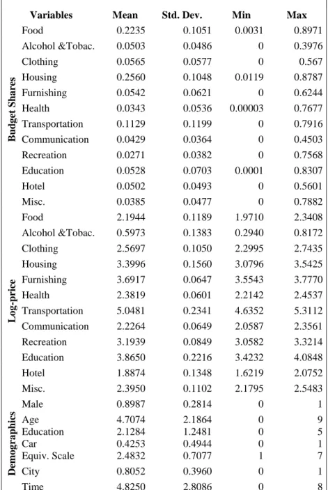
Monthly consumer price indexes for each of the consumption categories were taken from TurkStat. Prices are normalized, thus price vectors facing the national prices index as at 2003 (100,100, …,100).Our estimation sample consists of observation of households with non-zero consumption for education and health expenditures. We only keep the households whose OECD-modified equivalence scale is between1 – 7We includes even observable demographic characteristics in the model: (1)sex dummy equal to one for each male householder, (2)the age of householder 0(16-24), 1 (25-29), 2 (30-34), …, 8 (60-64), 9 (+65), (3)the education of householder 0 (illiterate), 1 (primary school), 2(secondary school), 3(high school), 4(college/university),5(master or PhD.), (4) OECD-modified equivalence scale (1 to 7), (5) a car-owner dummy equal to 1, (6) a time variable which represents the current year minus 2003 (it is zero for 2003) and(7) residential dummy equal to 1ifhousehold lives incity area which has more than 30000 inhabitants. Time variable is included in the model to take in the effect of potential adjustments changing with time such as tastes, quality. Table 1 summarizes statistics of our estimation sample, consisting of 7904 observations.

(4)

Table 1. Data Descriptive

Variables Mean Std. Dev. Min Max

B ud g et Sh a re s Food 0.2235 0.1051 0.0031 0.8971 Alcohol &Tobac. 0.0503 0.0486 0 0.3976 Clothing 0.0565 0.0577 0 0.567 Housing 0.2560 0.1048 0.0119 0.8787 Furnishing 0.0542 0.0621 0 0.6244 Health 0.0343 0.0536 0.00003 0.7677 Transportation 0.1129 0.1199 0 0.7916 Communication 0.0429 0.0364 0 0.4503 Recreation 0.0271 0.0382 0 0.7568 Education 0.0528 0.0703 0.0001 0.8307 Hotel 0.0502 0.0493 0 0.5601 Misc. 0.0385 0.0477 0 0.7882 L o g -price Food 2.1944 0.1189 1.9710 2.3408 Alcohol &Tobac. 0.5973 0.1383 0.2940 0.8172 Clothing 2.5697 0.1050 2.2995 2.7435 Housing 3.3996 0.1560 3.0796 3.5425 Furnishing 3.6917 0.0647 3.5543 3.7770 Health 2.3819 0.0601 2.2142 2.4537 Transportation 5.0481 0.2341 4.6352 5.3112 Communication 2.2264 0.0649 2.0587 2.3561 Recreation 3.1939 0.0849 3.0582 3.3214 Education 3.8650 0.2216 3.4232 4.0848 Hotel 1.8874 0.1348 1.6219 2.0752 Misc. 2.3950 0.1102 2.1795 2.5483 Demo g ra ph ics Male 0.8987 0.2814 0 1 Age 4.7074 2.1864 0 9 Education 2.1284 1.2481 0 5 Car 0.4253 0.4944 0 1 Equiv. Scale 2.4832 0.7077 1 7 City 0.8052 0.3960 0 1 Time 4.8250 2.8086 0 8

Source: HBS data, author’sanalysis

4. Methodology

We use the Lewbel and Pendakur’s EASI (2009) model to determine household demand functions. EASI demand system encloses a utility-derived model and nonlinear Engel Curves. This model has an advantage of providing more flexibility to the demand specification. Lewbel and Pendakur (2009) argued that classical parametric demand models such as AIDS, and other linear or quadratic versions of

(5)

demand models cannot include shape diversities and are controlled by Gorman (1981) type rank limitations. Furthermore the EASI demand system enables to measure of socioeconomic variation between household consumption. In addition, this model takes into consideration the unobserved preference heterogeneity through error term of the model. In general, model error terms cannot be illustrated as a represent for unobserved heterogeneity in many consumer demand models (Lewbel and Pendakur, 2009).

In order to sort the linear problem of Engel Curve and heterogeneities between the households out we setup the EASI models as recommended by Lewbel and Pendakur (2009). Through the EASI model we use substituting implicit utility functions into to the Hicksian budget shares, which yields the implicit Marshallian budget shares:

𝑤𝑗_{= ∑} _𝑏

𝑟𝑦𝑟+ 𝐶𝑧 + 𝐷𝑧𝑦 + ∑𝐿𝑙=0𝑧𝑙𝐴𝑙𝑝 𝑅

𝑟=0 + 𝐵𝑝𝑦 + 𝜀 (1)

The EASI budget shares (1) have compensated price effects conducted by 𝐴𝑙, 𝑙 =

0,1,2, … , 𝐿,andB, that allows for flexible price effects and for flexible interactions of these effects with expenditure and with observable demographic characteristics. In the model, the Engel curve terms 𝑏𝑟, 𝑟 = 0,1,2, . . . , 𝑅define budget shares as

Rth-orderpolynomials iny,where y is affine in lognominal expendituresx. This leads to Engel curves to have very complex shapes. Some analytically popular demand function shave budget shares quadratic in log total expenditures, corresponding to𝑟 = 0,1,2.At this point, we picked up the higher moments 𝑟 = 6, 7, which are statistically significant, and inserted into the model. The terms C and D enable demographic characteristics to enter budget shares through both intercept and slopetermson y. The random utility parameters, representing unobserved preference heterogeneity, as simple additive errors in the implicit Marshallian demand equations. Approximated nominal expenditures decreasing according to the Stone Price Index: that is, replace ywith 𝑦̃ defined by

𝑦̃ = 𝑥 − 𝑝′𝑤̅ (2)

Where𝑤̅ is the set of budget shares, x is nominal expenditures. When we compare to Equation (2), we obtain

𝑤𝑗_{= ∑} _𝑏

𝑟𝑦̃𝑟+ 𝐶𝑧 + 𝐷𝑧𝑦̃ + ∑𝐿𝑙=0𝑧𝑙𝐴𝑙𝑝 𝑅

𝑟=0 + 𝐵𝑝𝑦̃ + 𝜀̃ (3)

Where 𝜀̃ = 𝜀 with 𝜀̃described to make Equation (3) which is the Approximate EASI model. Five types of budget share elasticities are calculated in Lewbel and Pendakur (2009):

I. The semi elasticities of budget shares, Ψ , are given by:

Ψ = ∑𝐿 𝑎𝑗𝑘𝑙

𝑙=1 𝑧𝑙+ ∑𝑗𝑘=1𝑏𝑗𝑘𝑦 (4)

II. The real expenditure semi-elasticities, ℵ, are given by:

ℵ = ∑𝑅𝑟=1𝑏𝑟𝑗𝑟𝑦𝑟−1+ ∑𝐿𝑙=1ℎ𝑙𝑗𝑧𝑙+ ∑𝑗𝑘=1𝑏𝑗𝑘𝑙𝑛𝑝𝑘 (5)

III. The semi elasticities with respect to observable demographics, ζ, are given by:

ζ = 𝑔_𝑙𝑗+ ℎ_𝑙𝑗𝑦 + ∑𝑗 𝑎𝑗𝑘𝑙_𝑙𝑛𝑝𝑘

𝑘=1 (6)

IV. The compensated quantity derivatives with respect to prices, Γ ,are given by:

Γ = W−1_{(Ψ + 𝜔𝜔}′_{) , whereW=diag (𝜔)} ₍₇₎

V. The compensated expenditures elasticities with respect to prices, S, are given

by:

(6)

There are two possible resources of endogeneity in EASI model (Li et al., 2015). The first of these, because budget share 𝑤𝑗is used to create real income y, and its polynomials are endogenous. However, Lewbel and Pendakur (2009) and Zhen et al. (2013) stated that this type of endogeneity will be numerically unimportant when an incomplete demand model is estimated. The second of these and the most important one, prices may be caused by measurement errors. For these reason, instrumental variables are used to avoid the endogeneity and measurement errors problem. Moreover, we apply method iterative three-stage least squares(I3SLS) integrated with instrumental variable. This method, which is suggested by Lewbel and Pendakur (2009), is a special version of a fixed-point based estimator advised by Dominitz and Sherman (2005).

5. Empirical findings

We analyze demand system with J=12 goods, we are able to exclude the last equation of health expenditure from the system and solely analyze the remaining system of J-1=11 equations. The parameters of health expenditure are then reparable from through the adding up constraint that budget shares sum up to one.

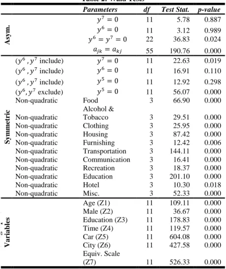
Firstly, symmetry restriction which means symmetry of𝐴𝑙 and B gives Slutsky

symmetry, is tested for in the model. We prefer to use %1 critical value for all tests due to having huge sample size (11 equations times 7904 observations per equation). Table 2 shows that the Wald test of symmetry in the asymmetric model is 190.76with a p-value <0.000. Hence we imposed the symmetry restriction on our model.

To specify the proper income polynomial’s degree, beginning from r=2, one higher degree of polynomial is included at a time and is analyzed the joint significance of the 𝑏𝑟 coefficients by minimum distance (Wooldrige, 2002:444; Zhen et al.,2013; Li

et al., 2015:239). Under the null that the 𝑅𝑡ℎ_{degree of the polynomial is exemptible}

and the test statistic is asymptotically distributed as𝜒2_{(𝐽 − 1). We also estimated a}

model with r=7 or 6.Both of these models are statistically insignificant with a p-value of 0.019 percent and 0.110 percent respectively. For this reason we offer further result for a symmetry-restricted model with r=0,1,…,5 using the I3SLS2_.

Iterative process has been converged in 1.10−11_{dimension that was suggested by}

Lewbel and Pendakur (2009) and Dominitz and Sherman (2005).

Turning to evidence of complicated Engel Curves shapes, we tested the argument that whether each of the eleven budgets shares equations could be reduced to a quadratic Engel curve. The results shows that except budget share of hotel expenditure which is slightly insignificant with a 0.018 percent p-value, rest of the budget shares are statistically significantly non-quadratic. These departures offer that allowing for complex Engel curves is useful property of EASI model.

2_{Seemingly Unrelated Regression (SUR) results are also available upon}

(7)

Table 2: Wald Tests

Parameters df Test Stat. p-value

Asy m . 𝑦 7_{= 0} ₁₁ _5.78 _0.887 𝑦6_{= 0} 11 3.12 0.989 𝑦6_{= 𝑦}7_{= 0} ₂₂ _36.83 _0.024 𝑎𝑗𝑘 = 𝑎𝑘𝑗 55 190.76 0.000 Sy mm et ric (𝑦6_{, 𝑦}7_include) _𝑦7_{= 0} ₁₁ _22.63 _0.019 (𝑦6_{, 𝑦}7_include) _𝑦6_{= 0} 11 16.91 0.110 (𝑦6_{, 𝑦}7_include) _𝑦5_{= 0} 11 12.92 0.298 (𝑦6_{, 𝑦}7_exclude) _𝑦5_{= 0} ₁₁ _56.07 _0.000 Non-quadratic Food 3 66.90 0.000 Non-quadratic Alcohol & Tobacco 3 29.51 0.000 Non-quadratic Clothing 3 25.95 0.000 Non-quadratic Housing 3 87.42 0.000 Non-quadratic Furnishing 3 12.42 0.006 Non-quadratic Transportation 3 144.11 0.000 Non-quadratic Communication 3 16.41 0.000 Non-quadratic Recreation 3 18.37 0.000 Non-quadratic Education 3 201.10 0.000 Non-quadratic Hotel 3 10.30 0.018 Non-quadratic Misc. 3 52.33 0.000 Demo g ra ph ic Va ria bles Age (Z1) 11 109.11 0.000 Male (Z2) 11 36.67 0.000 Education (Z3) 11 178.83 0.000 Time (Z4) 11 119.57 0.000 Car (Z5) 11 604.08 0.000 City (Z6) 11 427.58 0.000 Equiv. Scale (Z7) 11 526.33 0.000

Source: Author’s analysis

To consider demographic characters, the Wald Test does not reject for all demographic variables used in the model (see Table 2).

Figures 1-11 present our estimated coefficients of Engel curves for a four-member family with a 44-year-old male householder living in the city without a car in 2003 and having 𝜀 = 0. For this family 𝑤 = ∑5𝑟=0𝑏𝑟𝑦𝑟. The base-period Engel curves for

households with different values of unobserved heterogeneity are equal except for being vertically shifted by 𝜀. In addition, these based-period Engel curves are descriptive for the shape of Engel curves in other price regimes because of other price vectors.

In figures 1-11, every single green circle symbolizes the median of the budget share for the considered percentile of total expenditure defined in abscissa. Black, blue and red curves correspond to three increasing levels of smoothing.

(8)

Figure 1

Estimated Food Shares

Figure 2

Estimated Alcohol & Tobacco Shares

Figures 1 and 2 show the Engel curve for food and alcohol&tobacco. Engel curves of food and alcohol & tobacco have almost linear shape. However, these share equations are statistically significantly non-quadratic(see table 2).

Figure 3

Estimated Clothing Shares

Figure 4

Estimated Housing Shares

Figures 3 through 8 give the clothing, housing, communication, recreation, education and hotel Engel curves. All six sets of estimates appear quadratic however as shown in Table 2, with the exception of the hotel equation, these are statistically significantly non-quadratic.

(9)

Figure 5

Estimated Communication Shares

Figure 6

Estimated Recreation Shares

Figure 7

Estimated Education Shares

Figure 8

Estimated Hotel Shares

Figure 9

Estimated Furniture Shares

Figure 10

(10)

Figure 11

Estimated Misc. Shares

Figures 9-11 show Engel curves for furniture, transportation and miscellaneous. These share equations take the shape of S, as stating in previous Engel curves studies (Blundell et al., 2007). There is very important lesson that we can draw from these figures. The demand functions of some goods become close to linear or quadratic Engel curves whereas when logging total expenditures, whilst the others such as furniture, transportation and miscellaneous are not in a quadratic form. This indicates that demand system rank (Gorman 1981: Lewbel 1991) is higher than three. Particularly previous Turkish household demand studies have failed to obtain ranks greater than three due to the fact that most of departures from linear equations are somewhat quadratic.

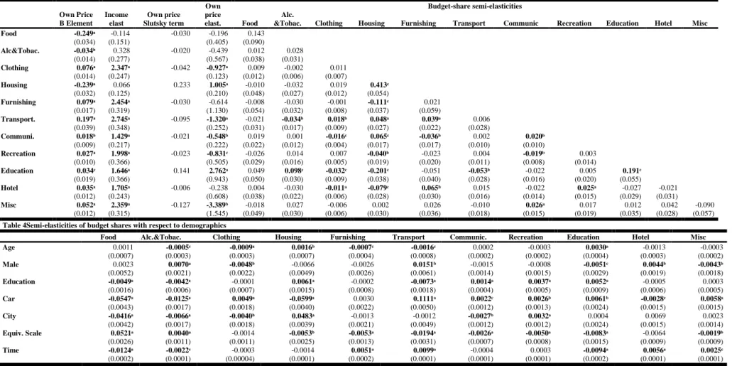
In the EASI model, price effects are easily evaluated considering the compensated (good-specific) expenditure elasticities, income elasticities or real income elasticities, compensated budget share semi-elasticities, and compensated quantity elasticities (Slutsky terms).Table 3 presents summary estimated price and income effects from the EASI demand model. The last column in the Table 3presents compensated price semi-elasticities for a reference family with median expenditure symmetry-restricted I3SLS estimates.

Considering the matrix of compensated budget share semi elasticities for the reference family at median expenditure given by 𝐴0, it can be seen that most of the

own price elasticities are huge and statistically significant. The own price compensated semi- elasticities for the rent budget share is 0.413. It can be interpreted that a rent price increases of 10 percent would be associated with a budget share 4.13percentage points higher when expenditure is raised to equate utility with that in the initial situation.

Several cross-price effects are also huge and statistically significant, offering that the substitution effect is crucial. For instance, the clothing budget share compensated communication cross price semi elasticity is -0.016, which means that an increase in the price of communication is associated with a significant decrease in the budget share for clothing, even after itis raised to hold the utility constant.

The fourth column of the Table 3 presents the own price expenditure elasticity with standard errors. The elasticity of compensated education expenditures is 2.762, and compensated rent expenditures is 1.005, respectively. On the other hand, the

(11)

elasticity of compensated misc. expenditures is -3.389. This value is highly negative and statistically significant as well.

The own price elasticities of rent and education expenditures is shown in the third column of Table 3.Although both of them are statistically significantly positive, this causes suspicion about global concavity (negative semi-definiteness) is violated. Global concavity of cost satisfies if and only if, the Slutsky matrix is negative semi- definite (Pollak and Wales, 1981).For the case 𝜀 = 0𝑗, the Slutsky matrix for the

reference family with median expenditure facing the base price is stated by the matrix 𝐴0 and the value of the Engel curve functions at median expenditure. In the

very first column of Table 3 the values of the own price Slutsky terms are illustrated. The own price Slutsky terms of rent and education are positive implying that global concavity is violated. Terrel (1996), Ryan and Wales (2000), Ogawa (2011), Li et al. (2015) consider that cost equations need onlyto pretend the assumptions of local concavity. Ogawa (2011) argues that cost equation just satisfies the local concavity as a result of increasing of land prices rapidly in the great growth of Japan’s economy caused by World War II. Li et al. (2015) reports almost the same results for China from 1995 to 2010. This phenomenon for soaring land prices is similar to Turkey after 2000. Therefore we analyze local concavity for data using the R code for EASI package as produced by Hoareau et al.(2012). The results present that the cost function is concave on more than 90% of the sample.

The leftmost column of estimates in Table 3 presents the estimated own price elements of B, which illustrates the magnitudes of the interactions between log total expenditures and own price. The estimated coefficient of the rent own price compensated semi elasticity on y is -0.239, and it is statistically significant. While the rent own price compensated semi elasticity for a reference family at the fifth percentile of expenditure is (x=2.746) for such a family at the ninety-fifth percentile of expenditure is (x=3.710). As stated above, its value at the median expenditure (𝑥 = 0) is 0.413. At the fifth percentile, its value is 0.413-(2.746 × 0.239) = -0.243. However, the value is 0.413-(3.710 × 0.239) = -0.473 at the ninety-fifth percentile. These results represent that rich households tend to less substitute than poor households when rent increase.

The second column of estimates in Table 3 shows income elasticities for the consumption bundles. Except for food, alcohol & tobacco and rent, income effects are huge and statistically significant. Therefore these expenditure bundles are luxury goods for the reference household.

Table 4 shows estimation of demographics variables elasticities for the consumption bundles with computed standard errors. Nearly all estimated elasticities are statistically significant and some of these elasticities are large. For example, when a household has a car, share of food and rent consumption reduces respectively 0.0547 and 0.0599; in contrast the share of transportation consumption increases 0.1111. For another example, when the household moves to the city area, share of food consumption reduces 0.0416; in contrast share of rent consumption increases 0.0483, maintaining the same utility level.

(12)

6. Conclusions

Lewbel and Pendakur (2009) provided an Exact Affine Stone Index (EASI) implicit Marshallian demand system, where utility is usually similar to an affine function of the log of expenditure reduced by the Stone Index. This EASI demand system is as adaptable in price response, as adjacent to linear in parameters and as easy to estimate as the Almost Ideal Demand (AID) system. Moreover, EASI system also allows for flexible interactions between prices and expenditures, and allows for any functional form for Engel curves, and permits error terms in the model to correspond to unobserved preference heterogeneity random utility parameters.

Owing to these advantages, we applied the EASI system based on the local concavity assumptions in order to analyze Turkish household consumer behavior. One of the significant indications of this study is that the rejection of linear or quadratic demand specification, which has been widely used on Turkish consumption data. The overall empirical statement of this work is that Engel curves, price and demographic elasticities are representative for households in Turkey. The results demonstrate that demographic characteristics will affect on household budget share structure, including education, age, gender and household equivalence scale, living in a city or urban area and having at least one car in the household.

This study has some limitations that need to be taken into account when interpreting the empirical results and could be useful addressed in further studies. First, the price data used in this work is not precise for all consumption categories for all Turkish households. We use monthly prices, which households came across in city area, from Turk Statas instrument variable. Second, our data does not include household wealth which might use as an instrument for a total expenditure for the future studies.

(13)

Turkish Households Consumption Behavior and Flexible Engel Curves 47 Table3Compensated Price Effects, Evaluated For Reference Type With Median Expenditure at Base Prices

Own Price B Element Income elast Own price Slutsky term Own price elast. Budget-share semi-elasticities Food Alc.

&Tobac. Clothing Housing Furnishing Transport Communic Recreation Education Hotel Misc Food -0.249ᵃ -0.114 -0.030 -0.196 0.143 (0.034) (0.151) (0.405) (0.090) Alc&Tobac. -0.034ᵇ 0.328 -0.020 -0.439 0.012 0.028 (0.014) (0.277) (0.567) (0.038) (0.031) Clothing 0.076ᵃ 2.347ᵃ -0.042 -0.927ᵃ 0.009 -0.002 0.011 (0.014) (0.247) (0.123) (0.012) (0.006) (0.007) Housing -0.239ᵃ 0.066 0.233 1.005ᵃ -0.010 -0.032 0.019 0.413ᶜ (0.032) (0.125) (0.210) (0.048) (0.027) (0.012) (0.054) Furnishing 0.079ᵃ 2.454ᵃ -0.030 -0.614 -0.008 -0.030 -0.001 -0.111ᶜ 0.021 (0.017) (0.319) (1.130) (0.054) (0.032) (0.008) (0.037) (0.059) Transport. 0.197ᵃ 2.745ᵃ -0.095 -1.320ᵃ -0.021 -0.034ᵇ 0.018ᵇ 0.048ᵃ 0.039ᵃ 0.006 (0.039) (0.348) (0.252) (0.031) (0.017) (0.009) (0.027) (0.022) (0.028) Communi. 0.018ᵇ 1.429ᵃ -0.021 -0.548ᵇ 0.019 0.001 -0.016ᶜ 0.065ᶜ -0.036ᵇ 0.002 0.020ᵇ (0.009) (0.217) (0.222) (0.022) (0.012) (0.004) (0.017) (0.017) (0.010) (0.010) Recreation 0.027ᵃ 1.998ᵃ -0.023 -0.831ᶜ -0.026 0.014 0.007 -0.040ᵇ -0.023 0.004 -0.019ᵇ 0.003 (0.010) (0.366) (0.505) (0.029) (0.016) (0.005) (0.019) (0.020) (0.011) (0.008) (0.014) Education 0.034ᶜ 1.646ᵃ 0.141 2.762ᵃ 0.049 0.098ᶜ -0.032ᶜ -0.201ᶜ -0.051 -0.053ᵇ -0.022 0.005 0.191ᶜ (0.019) (0.366) (0.943) (0.050) (0.030) (0.009) (0.038) (0.040) (0.028) (0.016) (0.020) (0.055) Hotel 0.035ᵃ 1.705ᵃ -0.006 -0.238 0.004 -0.030 -0.011ᵃ -0.079ᶜ 0.065ᵇ 0.015 -0.022 0.025ᵃ -0.027 -0.021 (0.012) (0.243) (0.608) (0.038) (0.022) (0.006) (0.028) (0.030) (0.016) (0.014) (0.015) (0.029) (0.031) Misc 0.052ᵃ 2.359ᵃ -0.127 -3.389ᵇ -0.018 0.027 -0.006 0.002 0.026 -0.010 0.026ᵃ 0.017 0.012 0.042 -0.090 (0.012) (0.315) (1.545) (0.049) (0.030) (0.006) (0.030) (0.036) (0.018) (0.015) (0.019) (0.035) (0.028) (0.057)

Table 4Semi-elasticities of budget shares with respect to demographics

Food Alc.&Tobac. Clothing Housing Furnishing Transport Communic. Recreation Education Hotel Misc

Age 0.0011 -0.0005ᶜ -0.0009ᵃ 0.0016ᵇ -0.0007ᶜ -0.0016ᶜ 0.0002 -0.0003 0.0030ᵃ -0.0013 -0.0003 (0.0007) (0.0003) (0.0003) (0.0007) (0.0004) (0.0008) (0.0002) (0.0002) (0.0004) (0.0003) (0.0002) Male 0.0023 0.0070ᵃ -0.0048ᵇ -0.0066 -0.0026 0.0151ᵇ -0.0015 -0.0008 -0.0051ᶜ 0.0044ᵇ -0.0043ᵇ (0.0052) (0.0021) (0.0022) (0.0049) (0.0026) (0.0061) (0.0014) (0.0015) (0.0029) (0.0019) (0.0018) Education -0.0049ᵃ -0.0042ᵃ -0.0001 0.0061ᵃ -0.0002 -0.0073ᵃ 0.0014ᵃ 0.0037ᵃ 0.0052ᵃ -0.0005 0.0003 (0.0016) (0.0006) (0.0007) (0.0015) (0.0008) (0.0018) (0.0004) (0.0005) (0.0009) (0.0006) (0.0005) Car -0.0547ᵃ -0.0125ᵃ 0.0049ᵃ -0.0599ᵃ 0.0030 0.1111ᵃ 0.0022ᶜ 0.0026ᵇ 0.0061ᵇ -0.0028ᶜ 0.0058ᵃ (0.0043) (0.0017) (0.0018) (0.0040) (0.0022) (0.0050) (0.0012) (0.0013) (0.0024) (0.0015) (0.0015) City -0.0416ᵃ -0.0066ᵃ -0.0040ᵇ 0.0483ᵃ -0.0013 -0.0012 -0.0027ᵇ 0.0032ᵃ 0.0004 0.0069 0.0023 (0.0042) (0.0017) (0.0018) (0.0039) (0.0021) (0.0049) (0.0012) (0.0012) (0.0024) (0.0015) (0.0014) Equiv. Scale 0.0521ᵃ 0.0040ᵃ -0.0014 -0.0053ᵇ -0.0053ᵃ -0.0194ᵃ -0.0026ᵃ -0.0050ᵃ -0.0083ᵃ -0.0064 -0.0019ᵇ (0.0026) (0.0011) (0.0011) (0.0025) (0.0013) (0.0031) (0.0007) (0.0008) (0.0015) (0.0009) (0.0009) Time -0.0124ᵃ -0.0022ᶜ -0.0003 -0.0014 0.0051ᵃ 0.0099ᵃ -0.0004 0.0003 -0.0094ᵃ 0.0056ᵃ 0.0025ᶜ (0.0002) (0.0001) (0.00004) (0.0001) (0.0002) (0.0001) (0.0001) (0.0001) (0.0002) (0.0001) (0.0001)

(14)

7. References

Akbay, Cuma (2005), Kahramanmaraş’ta Hanehalklarının Gıda Tüketim Talebi Ekonometrik Analizi.KSÜ Fen ve Mühendislik Dergisi, 8(1), 114–121. Akbay, C., Boz, I. Chern, W.S. (2007). Household FoodConsumption in Turkey.

European Review of Agricultural Economics, 34(2), 209–231, DOI:

10.1093/erae/jbm011

Blundell, R.; Browning, M.; Crawford I. A.(2003). Nonparametric Engel

CurvesandRevealedPreference.Econometrica, 71(1), 205–240,

DOI: 10.1111/1468-0262.00394

Blundell, R.; Chen, X; Kristensen, D. (2007). Semi-Nonparametric IV Estimation of Shape-Invariant Engel Curves.Econometrica, 75(6), 1613–1669, DOI: 10.1111/j.1468-0262.2007.00808.x

Bilgiç, A., Yen, Steven T. (2013), Household Food Demand in Turkey: A Two-Step

Demand System Approach.Food Policy, 43, 267–277.

doi:10.1016/j.foodpol.2013.09.004

Dominitz, J., Sherman, R. P. (2005).Some Convergence Theory for Iterative Estimation Procedures with an Application to Semiparametric

Estimation.Econometric Theory, 4, 838–863, DOI:

10.1017/S0266466605050425

Fidan, H., Klasra, A. M. (2005). Seasonality in Household Demand for Meat and

Fish : Evidence from an Urban Area.Turkish Journal of

Veterinary&AnimalSciences, 29, 1217–1224.

Fisunoğlu, M. H., Sengul, S. (2011). Adana Kentsel Alanda Hanehalkı Tüketimi.Çukurova Üniversitesi Sosyal Bilimler Enstitüsü Dergisi, 20(1), 251–266.

Gorman, W. M. (1981).Some Engel Curves, Deaton, Angus (Ed), Essays in the Theory and Measurement of Consumer Behaviour in Honor of Sir Richard Stone, Cambridge, Cambridge University Press.

Günden, C.; Bilgiç, A.; Miran, B.; Karlı, B. (2011). A Censored System of Demand Analysis to Unpacked and Prepackaged Milk Consumption in Turkey.Quality&Quantity, 45(6), 1273–1290. doi:10.1007/s11135-011-9501-6

Hoareau, S., Lacroix, G., Hoareau, M., &Tiberti, L. (2012).Exact Affine Stone Index Demand System in R: The EASI Package. Technical Report, University of Laval.

Howe, H. (1977). Cross-Section Application of Linear Expenditure Systems: Responses to Sociodemographic Effects..American Journal of Agricultural Economics, 59(1), 141–148.

İpek, E. (2014), Hanehalkı Tüketim Davranışlarını Ölçmeye Yönelik Talep Sistemi

Teorileri ve Türkiye Üzerine Bir Uygulama. Unpublished PhD. Thesis,

Karadeniz Technical University, Trabzon, Turkey.

Koç, A., Alpay, S. (2002), Household Demand in Turkey: An Application of Almost Ideal Demand System with Spatial Cost Index, Economic Research

Forum Working Papers No: 0226, 1–14.

Koç, A., Yurdakul, O. (1995). Türkiye’de Gıda Harcamaları ve Harcama Esneklikleri. Çukurova Üniversitesi Ziraat Fakültesi Dergisi, 10(3), 175– 188.

Lewbel, A. (1991). The Rank of Demand Systems : Theory and Nonparametric Estimation. Econometrica, 59(3), 711–730, DOI: 10.2307/2938225

(15)

Lewbel, A., Pendakur, K. (2009). Tricks with Hicks: The EASI Demand System.The

American Economic Review, 827-863, DOI:10.2139/ssrn.913080

Li, L., Song, Z., Ma, C (2015). Engel Curves and Price Elasticity in Urban Chinese

Households.Economic Modeling, 44, 236–242,

DOI:10.1016/j.econmod.2014.10.002

Nisanci, M. (1998), Türkiye’de Tüketici Harcamalarının Analizi- İdeale Yakın Talep

Sistem Uygulaması.Unpublished PhD. Thesis, Atatürk University, Erzurum,

Turkey.

Nisanci, M. (2003), “Hanehalkı Harcamalarının Engel Eğrisi Analizi: 1994 Türkiye Kentsel Kesim Örneği.” İstanbul Üniversitesi Siyasal Bilgiler Fakültesi

Dergisi (28), 155-167.

Ogawa, K. (2011), “Why are Concavity Conditions Not Satisfied in The Cost Function? The Case of Japanese Manufacturing Firms during the Bubble Period.” Oxford Bulletin of Economics and Statistics 73(4), 556-580, DOI: 10.1111/j.1468-0084.2010.00623.x

Özçelik, A.; Şahinli, M.A. (2009). Estimating Elasticities with the Almost Ideal Demand System: Turkey Results.The International Journal of Economic

and Social Research, 5(2), 12–23.

Pollak, R. A.,Wales, T. J. (1981). Demographic Variables in Demand Analysis.Econometrica, 49(6), 1533–1551. DOI: 10.2307/1911416

Ryan, D.L., Wales, T. J. (2000). Imposing Local Concavity in the Translog and Generalized Leontief Cost Functions. Economics Letters, 67(3), 253-260, DOI: 10.1016/S0165-1765(99)00280-3

Selim, R. (2000), “Türkiye’de Tüketim Harcama Kalıpları: 1994,”in Halil Aksu’ya Armağan, İstanbul Teknik Üniversitesi İşletme Fakültesi, 109-121.

Sengul, S.,Sigeze, C. (2013).Türkiye’de Hanehalkı Tüketim Harcamaları : Pseudo Panel Veri ile Talep Sisteminin Tahmini.Paper presented at International Conference on Eurasian Economies Russia.

Sengul, S., Tuncer, I. (2005). Poverty Levels and Food Demand of The Poor in Turkey.Agribusiness, 21(3), 289–311. DOI:10.1002/agr.20049

Şahinli, M. A. (2010). Yaklaşık İdeal Talep Analizi Yöntemi ile Harcama ve Fiyat Esnekliklerinin Tahmini.Eskişehir Osmangazi Üniversitesi İİBF Dergisi,

5(2), 147–158.

Sahinli, M. A. (2013). The Turkish Demand forFood. Turkish Studies, 8, 2111– 2118.

Stone, R. (1954). Linear Expenditure Systems and Demand Analysis: An Application to the Pattern of British Demand. The Economic

Journal, 64(255), 511-527. DOI: 10.2307/2227743

Tekgüç, H. (2012). SeparabilityBetweenOwnFoodProductionandConsumption in Turkey.Review of Economics of theHousehold, 10(3), 423–439. doi:10.1007/s11150-011-9126-5

Terrell, D. (1996). Incorporating Monotonicity and Concavity Conditions in Flexible Functional Forms.Journal of Applied Econometrics, 11(2), 179-194. TURKSTAT. Household Budget Survey, 2003–11. Ankara: Turkish Statistical

Institute.

Wooldridge, J. M. (2010), Econometric Analysis of Cross Sectionand Panel Data, MIT press.

(16)

Zhen, C., Finkelstein, E. A., Nonnemaker, J. M., Karns, S. A., Todd, J. E. (2013). Predicting the Effects of Sugar-Sweetened Beverage Taxes on Food and Beverage Demand in a Large Demand System.American Journal of