Can unemployment cured by economic growth and foreign direct investment?

CAN UNEMPLOYMENT BE CURED BY ECONOMIC

GROWTH AND FOREIGN DIRECT INVESTMENT?

İsmail AKTAR*

Nedret DEMİRCİ**

Latif ÖZTÜRK***

Abstract

This study applies the VAR technique of variance decomposition and impulse response function analysis to investigate various interrelationships among foreign direct investment (FDI), exports (EX), unemployment (UR) and gross domestic product (GDP) in the case of Turkey over the period 2000:1 to 2007:4. We find that there are two cointegrating vectors in the system, indicating there is long run relationship. Our findings show that FDI did not have any contribution to reduce the unemployment rate in Turkey. Variations in EX have a positive impact on GDP but they are insignificant. Therefore, this study does not support the export led economic growth model. Variation in GDP does not reduce the unemployment rate either.

Özet

Bu çalışma VAR modeli kullanılarak doğrudan yabancı sermaye ve (FDI), ihracat (EX), işsizlik (UR) ve gayrı safi milli hasıla arasındaki ilişkileri dönemlik (2000:1-2007:4) veri kullanarak incelemeyi amaçlamaktadır. Sistemde iki eşbütünleşik seri bulunmuştur. Bu uzun dönem ilişkinin varlığını ispatlamaktadır. Ancak, doğrudan yabancı sermaye yatırımla-rının istihdamı arttırmadığı ortaya konmuştur. İhracattaki varyasyonlar GDP üzerindeki etkisi her ne kadar pozitifse de istatistiksel olarak anlamlı değildir. Bu durum ihracat büyümeli ekonomik modeli desteklememektedir. Son olarak GDP gelişmeler anılan dönemde işsizliği azaltıcı yönde bir etki yaratmamışlardır.

Key words: Foreign direct investment, VAR, economic growth, export

JEL classification: O16

* _{Faculty of Economics and Administrative Sciences, Kırıkkale University.} ** _{Faculty of Economics and Administrative Sciences, Kırıkkale University.}

Introduction

As the globalization spreads out in the world, some countries try to be-nefit of this. No doubt that globalization makes cheaper obtaining capital via foreign direct investment (FDI). Turkey has also been interested in having FDI in order to improve her economic development since 1980s. FDI can contribute to Turkey’s foreign trade, industrialization, and human resources. The literature argues in two ways that FDI can create significant impact on countries capital formation, international trade, economic growth and emp-loyment. On the other hand, some literature emphasizes that FDI has no contribution to economic growth or employment of the host country.

Since 1980 Turkey also changed its economic structure completely and moved from import substitution economy to export-led economic growth model. Although FDI was supposed to be a leading factor in economic growth, it could not play a significant role till 2001. The reason might be mainly political instability in Turkey and the world economic situation. Yet, the one party ruling brought political stability since 2002 election and this made Turkey attractive for foreign investors again. The organization of the article is as fallows: the fallowing section gives some literature review and brief detail about Cheng’s model that we use, the second section explains concerned macroeconomic variables in Turkey, the third section is data and methodology, the fourth section empirical results and finally some conclu-ding remarks.

1. Literature Review

This paper fallows the Cheng’s article about Taiwan et al. (2006). We basically applied the same model to Turkey with some modifications. Cheng discusses in the article et al. (2006) some studies done regarding Taiwan. The author basically divides the literature into five categories. First one talks about that the explanation of FDI could be economic growth and external trade. The second deals with the positive or negative relationship between FDI and export. The fourth one gives even more contradictory results that FDI and export have positive impact on economic growth in some research and have negative impact in others. The fifth one basically analyzes the Okun’s law. It concludes that there is a negative correlation between unemp-loyment and economic growth in imperfect competition. Further discussion can be obtained from Cheng’s article et al. (2006).

Cheng and Ku (2000) investigated whether FDI has any impact on in-vesting firms’ growth using Taiwan’s data. They found that FDI supports the domestic industries and trade yet has no positive impact on employment.

Grinols (1991) emphasizes that in order to have welfare gains the wa-ges in new capital sectors must be relatively higher than the wawa-ges in the other sectors. Fang, Zeng, Zhu (1999) studied the effect of FDI on urban employment, labor income and national welfare. They utilized the Harris-Todaro economic model. They showed the conditions that as the FDI inf-lows, its impact on economic factors mentioned above.

Zhao (1998) investigated the relationship between FDI and unemploy-ment and wage rates. He found that FDI reduces the unionized labor wage rate. When union concerns more about the employment than wages, then FDI reduces the unionization rate in ununionized sector.

Bailey and Driffield (2006) focuse on the impacts of FDI, trade, techno-logical development on skilled and unskilled workers in UK. They utilize the panel data in small business and contrast the findings with British industrial policy. They found skilled workers enjoy the advantage of FDI and trade, unskilled workers are worse off due to the FDI and trade. At the end they conclude that UK might consider her industrial policy.

Barros and Cabral (2000) search whether there is a competition among the countries for attracting FDI: Their results suggest that FDI prefers to go to a country where there is high unemployment.

Braconier and Ekholm (2000) argue that capital inflows have an ambi-guous impact on unemployment rate. It is so because the activities could be complementary or substitutability between foreign and domestic producti-ons.

Eckel (2003) analyzes FDI effects on employment from the high wage country’s perspective. Findings indicate that employment effect depends upon the substitution of domestic labor by foreign labor and cost savings. Hence, the impact of FDI on domestic employment relies on internationality of production and the mobility of capital.

Brady and Wallace (2000) investigated the effect of FDI on employ-ment and labor income in US for the period 1978-1996 under the spatializa-tion theory. Their findings are consistent with the theoretical work that sug-gests FDI adversely effect the employment and labor income in US for the concerned period.

Taban and Aktar (2005) investigated the export-led growth hypothesis covering the data from 1923 to 2003. They investigate whether there exists any cointegration between export and economic growth using Johansen test technique. Even though the results did not support the idea that export growth Granger causes the GDP growth in the closed economy (i.e. between 1923-1980) period they found a bidirectional causal relationship between the export growth and the GDP growth for only open economy period (i.e. after 1980) in the short-run.

Although the literature provides some useful relationship between eco-nomic growth and export or unemployment, it does not give the causal links between FDI, exports, economic growth and unemployment based on a mul-tivariate framework. This paper is another attempt to see the link between FDI exports, economic growth and unemployment in Turkey based on a multivariate framework. We utilize an impulse response function and vari-ance decomposition to analyze the short-run dynamic response of the macro-economic variable series mentioned above, and cointegrating test to deter-mine whether there exist a long-run equilibrium relationship among the vari-ables.

2. Foreign Direct Investment, Export, Economic Growth and Unemployment in Turkey

Political climate in Turkey has been ups and downs since 1980. One party rule lasted almost 10 years in which Turkey really experienced radical reforms in economical and political arenas. Unfortunately, 1990s was coali-tion years and Turkey could not maintain reforms. After the 2001, when the worst crises ever happened in Turkish economic history, the early election brought one party rule again and EU oriented reforms accelerated one more time. Most of the macroeconomic variables showed the recovery of the Tur-kish economy apart from unemployment.

Even though there were some attempts to boost the FDI in Turkey from time to time, the significant amount had not occurred since 2001. From the historical point of view, the Foreign Investment Encouragement Act was passed in 1954. This law was replaced by better one in 2003. The new act does not require foreigners to take permission for the investment in Turkey. Republic of Turkey also accepts the international court against confiscation of foreign investment. As Acikalin (2007) discusses that FDI began to

inf-low to country after 1980 due to export led growth model. However, 1990s were missing years regarding FDI in Turkey. For instance, in 1985, FDI was only 99 million US dollars. Five years later it reached at 684 million US dollars. When we came to the year 2001 the FDI jumped into 3,266 million US dollars. After that, FDI grew steadily until now. The latest figure was 18,420 million US dollars in 2007 according to Turkish Treasury Depart-ment.

Although there has been significant improvement in FDI, Turkey has still very low portion of the total FDI in the world. During 1992-1997 Tur-key’s share was only 0.24 percent at average. When we compare Turkey with other developing countries, she could manage to receive only around 1 percent.

The composition of FDI in Turkey also reflects her foreign trade com-position. Turkey’s biggest trade partner is EU. This is also the case of FDI. 55 percent of foreign companies belong to the members of EU.

Turkey’s export became an important subject after 1980. Before that time Turkey’s policy was import-substitute economy. 1980s brought export-led growth model. For instance while Turkey’s total export was only 2 bil-lion US dollars in 1980, it reached at almost 13 bilbil-lion US dollars in 1990, it became around 28 billion US dollars and finally it was more than 107 billion US dollars in 2007. No doubt export growth has been tremendous since 1980.

The unemployment rate (UR) was always high for Turkey during the concerned period of time. It was around 8 percent till 2001 and after that it went up to around 10 percent and persisted since then. Even though there has been steady economic growth in recent years, unemployment rate has not fallen at all. Unemployment is a great concern of the public as well as go-vernment.

3. Data and Methodology

We have four variables; foreign direct investment (FDI) in US dollars, gross domestic product (GDP) at current prices in US dollars, export (EX) at current prices in US dollars, and unemployment rate (UR). The data runs through 2000:1 to 2007:4. We choose this range due to the fact that FDI and export became an important subject for Turkey around that time.

Particu-larly, when we look at the FDI, the figures are pretty small in the economy before 2000. Unlike Cheng et. al. (2006), we did not employ outflow FDI since the Turkish outflow FDI figures are negligible. The data are quarterly and come from several sources; the Department of Treasury, Central Bank, The State Planning Organization and Statistical Institute of Turkey. We take the log values of all variables.

In the VAR model all variables are explained by their lagged values and other variables lagged values.

The VAR of order p model can be expressed in matrix representation as follows:

lnYt=Ψ+ Θ1 lnYt-1 +. . . Θp lnYt-p +vt; =1, . . . .,N (1)

where ln Yt = ⎥ ⎥ ⎥ ⎥ ⎥ ⎥ ⎦ ⎤ ⎢ ⎢ ⎢ ⎢ ⎢ ⎢ ⎣ ⎡ t t t t t GR GNP EX UR FDI ln ln ln ln ln Ψ= ⎥ ⎥ ⎥ ⎥ ⎥ ⎥ ⎦ ⎤ ⎢ ⎢ ⎢ ⎢ ⎢ ⎢ ⎣ ⎡ Ψ Ψ Ψ Ψ Ψ 5 4 3 2 1 i

Θ

= ⎥ ⎥ ⎥ ⎥ ⎥ ⎥ ⎦ ⎤ ⎢ ⎢ ⎢ ⎢ ⎢ ⎢ ⎣ ⎡ Θ Θ Θ Θ Θ Θ Θ Θ Θ Θ i i i i i i i i i i 55 , 45 , 35 , 25 , 15 , 51 , 41 , 31 , 21 , 11 .... vt= ⎥ ⎥ ⎥ ⎥ ⎥ ⎥ ⎦ ⎤ ⎢ ⎢ ⎢ ⎢ ⎢ ⎢ ⎣ ⎡ t 5, t 4, t 3, t 2, t 1, v v v v v

In the equation above Ψ and Θi (i=1,…,p) are VAR parameters to be

estimated and vt is random errors with zero mean and finite variance.

We aim at finding how each variable response is shocked by other vari-ables of the system. Hence, using impulse response function and variance decomposition provides us short run dynamic relationship between UR and other macroeconomic variables in the VAR equation. Each variable’s res-ponse over time and other variables effects can be seen via impulse resres-ponse function. Thus, we should plot the impulse response functions. The forecast

error of variance decomposition analysis allows us to draw conclusion about the movement in sequence due to its own shocks versus shocks to other vari-ables.

Before we apply to cointegrating test, we should check whether each series is stationary or not. Thus, we utilize the unit root test of augmented Dickey-Fuller (ADF) test statistics. Furthermore, ADF test gives us the order of integration of economic time series. Dickey and Fuller (1979) explained that if the series is non-stationary the null hypothesis representing a unit root cannot be rejected. Thus, we should take first or higher differencing to eli-minate the unit root accordingly. Akaike’s Information Criterion gives us the optimum lag-length.

If there is cointegration, then we can apply to VAR model. The inverse of VAR model into a moving average representation gives us impulse res-ponses and variance decomposition of forecast-error. Sims (1980) gives us the reduced form of the VAR as vector moving-average representation as fallows:

I

C

C

C

Y

i i t i i i t

=

Φ

+

=

Δ

∑

∑

∞ = − ∞ =0 0 0

;

ln

_ε

(2)

where ∆ indicates first difference and Ci is A coefficient matrix.

when applying Cholesky decomposition, a vector moving average rep-resentation is

∑

∑

∞ = − ∞ =

+

Φ

=

Δ

0 ' 0

)

)(

(

ln

i i t i i i t

C

C

P

P

Y

_ε

(3)

where P is the inverse of the lower triangular Cholesky factor of the

re-sidual covariance matrix and PP’=∑.

There are two different ways in cointegration test: Engle and Granger (1987) based on single equation and Johansen (1988) based on systems of equation. Engle and Granger (1987) test the stationary of residuals based on single-equation static regression of one variable. Thus, Johansen (1988) es-timation technique is better in the sense that it uses maximum likelihood of a

full system that provides test of λmax and Trace statistics to determine the

Jo-hansen and JoJo-hansen and Jesulius (1990) estimation technique to determine the cointegration and the number of cointegrating vectors.

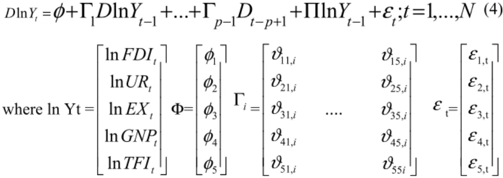
Thus, the restricted VAR based on Johansen (1988) and Johansen and Jesulius (1990) model with differences and error correction derived from the cointegration equation is as fallows:

N

t

Y

D

Y

D

_{t p t p t t} Y Dln t =

φ

+

Γ

₁

ln

₋₁

+

...

+

Γ

_{−1 − +1}

+

Π

ln

₋₁

+

ε

;

=

1

,...,

(4) where ln Yt = ⎥ ⎥ ⎥ ⎥ ⎥ ⎥ ⎦ ⎤ ⎢ ⎢ ⎢ ⎢ ⎢ ⎢ ⎣ ⎡ t t t t t TFI GNP EX UR FDI ln ln ln ln ln Φ= ⎥ ⎥ ⎥ ⎥ ⎥ ⎥ ⎦ ⎤ ⎢ ⎢ ⎢ ⎢ ⎢ ⎢ ⎣ ⎡ 5 4 3 2 1

φ

φ

φ

φ

φ

i

Γ

₌ ⎥ ⎥ ⎥ ⎥ ⎥ ⎥ ⎦ ⎤ ⎢ ⎢ ⎢ ⎢ ⎢ ⎢ ⎣ ⎡ i i i i i i i i i i 55 , 45 , 35 , 25 , 15 , 51 , 41 , 31 , 21 , 11 ....

ϑ

ϑ

ϑ

ϑ

ϑ

ϑ

ϑ

ϑ

ϑ

ϑ

ε

_t= ⎥ ⎥ ⎥ ⎥ ⎥ ⎥ ⎦ ⎤ ⎢ ⎢ ⎢ ⎢ ⎢ ⎢ ⎣ ⎡ t 5, t 4, t 3, t 2, t 1,

ε

ε

ε

ε

ε

D shows the difference operator Γi represents adjustment of the short run.

The matrix _{Π is potentially reduced rank γ(γ is the number of cointegrating}

vectors or the rank) and thus Π=αβI _{where α (the matrix of adjustment}

co-efficients in the restricted VAR model) and β (the matrix of cointegrating

vectors) are 5xγ matrices of full ranks. The matrix Π=αβI _{indicates the long}

run relationship between Yt variables and the rank of Π is the number of

linearly independent and stationary linear combinations of variables.

4. Empirical Results

We start with checking whether our macro series are stationary by applying ADF test. We use Eviews-5 econometric program. The ADF test results for unit root with the levels and first differences of the variables are given in Table 1.

Table 1. Augmented Dickey-Fuller (ADF) tests

lnUR lnGDP lnEX lnFDI

Levels of the variables

T

τ

-3.09 -2.30 -2.37 -2.22

First differences of the variables

T

τ

-9.62* -4.80** -3.65** -7.38*

The optimal lag in the cointegrating test was selected by minimizing the Akaike information criterion Table 1 shows the ADF results with trend and intercept. As it can be seen that we fail to reject the null hypothesis that all series contain unit root. Yet, when we take the first difference, all the series become stationary. Therefore, all the series are integrated of order one I(1).

Since the variables are stationary and integrated order of one, we emp-loy cointegration technique of Johansen et al. (1988) and Johansen and Juse-lius et al. (1990) to test whether there exist a long-run relationship among variables. Johansen’s maximum likelihood method tests the null hypothesis that states there is no cointegration. The cointegrating ranks of the variables

are tested using λmax statistic. The test result for cointegrating rank is

repor-ted in Table 2.

Table 2. Result of the cointegration tests (VAR lag=2)

Eigenvalue H0 H1 Trace test

λ

max test Critical value 1%(Trace) Critical value 1%(

λ

_max) 0.89 r=0

r

≥

1

107.08* 62.00* 63.87 32.11 0.70

r

≤

1

r

≥

2

45.08* 33.26* 42.91 25.82 0.28

r

≤

2

r ≥3 _{11.82 9.20 25.87} 19.38 0.09 r≤3

r

≥

4

2.61 2.61 12.51 12.51 Estimated vectors cointegrating

lnUR lnGDP lnEX lnFDI

1 0 1.06 0.06

(0.46) (0.02)

0 1 0.64 -0.07

(0.86) (0.04)

* denotes significance at %1 level r indicates the number of cointegrating vectors

The optimal lag in the cointegrating test was selected by minimizing the Akaike information criterion Numbers in parentheses are the standard error value

Table 2 shows the cointegrating test results. Since calculated λmax (=62.00) and Trace (=107.08) are above the critical values (32.11) and (63.87) respectively at 1 percent, we can clearly reject the null hypothesis stating there is no cointegration. Furthermore, the second null hypothesis stating one versus two cointegrating vectors, we also reject the null

hypothe-sis since the calculated λmax (=33.26) and Trace (=45.08) are above the

critical values (25.82) and (42.91) respectively. However, when it comes to two cointegrating vectors vs. three cointegrating vectors, we fail to reject the

null hypothesis since the calculated λmax (=9.20) and Trace (=11.82) are

below the critical values (19.38) and (25.87) respectively. Hence, we conc-lude that we have two cointegrating vectors in our system. Furthermore, Eviews-5 also reports the normalized cointegrating vectors. According to the normalized cointegrating vectors, export and foreign direct investment have a negative but not significant impact on unemployment rate. The sign do not match with our theoretical expectation. Export has a positive significant impact on GDP while foreign direct investment has a negative impact on GDP, which is inconsistent with our theoretical expectation. Thus we can conclude that due to the co-movement among the variables there exists a long run relationship.

Since we have established the long run relationship among the relevant time series, we can estimate the restricted VAR with error correction term. First difference can be estimated by inverting the VAR into a moving avera-ge representation, and consequence the impulse responses and variance de-composition can be found. The optimum lags will be chosen based on Akai-ke information criterion.

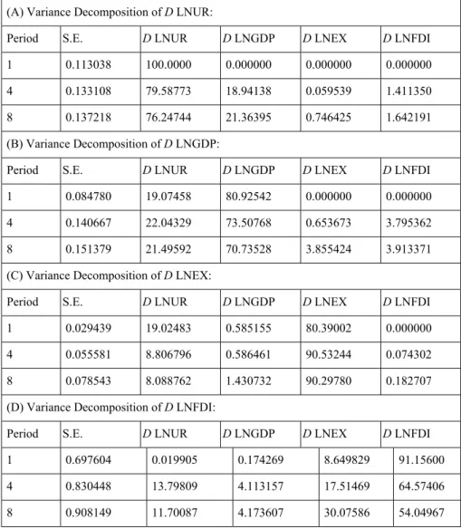
We apply the variance decomposition to see that the forecast error components of one variable originating from the orthogonalized innovations of the system. Variance decomposition enables us to distinguish the relative importance of the economic variables in the models. Estimated results are shown in Table 3.

Table 3. Variance decomposition percentage analysis

(A) Variance Decomposition of D LNUR:

Period S.E. D LNUR D LNGDP D LNEX D LNFDI 1 0.113038 100.0000 0.000000 0.000000 0.000000 4 0.133108 79.58773 18.94138 0.059539 1.411350 8 0.137218 76.24744 21.36395 0.746425 1.642191 (B) Variance Decomposition of D LNGDP:

Period S.E. D LNUR D LNGDP D LNEX D LNFDI 1 0.084780 19.07458 80.92542 0.000000 0.000000 4 0.140667 22.04329 73.50768 0.653673 3.795362 8 0.151379 21.49592 70.73528 3.855424 3.913371 (C) Variance Decomposition of D LNEX:

Period S.E. D LNUR D LNGDP D LNEX D LNFDI 1 0.029439 19.02483 0.585155 80.39002 0.000000 4 0.055581 8.806796 0.586461 90.53244 0.074302 8 0.078543 8.088762 1.430732 90.29780 0.182707 (D) Variance Decomposition of D LNFDI:

Period S.E. D LNUR D LNGDP D LNEX D LNFDI 1 0.697604 0.019905 0.174269 8.649829 91.15600 4 0.830448 13.79809 4.113157 17.51469 64.57406 8 0.908149 11.70087 4.173607 30.07586 54.04967

Table 3 indicates that the reported numbers indicate the percentage of forecast error in each variable that can be attributed to innovations in other variables in three different time horizons: first period (one quarter), fourth period (one year) and eighth period (two years).

The part A of Table 3 indicates that the innovation of unemployment rate is due to its own innovation starting from 100 % in the first quarter to 76 % up to eight quarter. Besides, changes in unemployment rate is also explai-ned by around 21 %, 1.6 %, and 0.7 by GDP, FDI and EX respectively in the

eighth quarter. This indicates that the innovation in unemployment is mainly explained by its own variation, and GDP, FDI and EX respectively.

When looking at the part B of Table 3, we see that in the first quarter the change in GDP is explained by 80% of its own shocks in the first quarter and it goes down to 70% in the eighth quarter. In the eighth quarter, however, the GDP variation is accounted of 21% by UR, 3.9% by FDI and only 3.8% by EX. Hence, the innovation of GDP is mainly explained by its own variation and UR, FDI and EX respectively.

Moreover, the part C of Table 3 indicates that the innovation of EX is exp-lained 80 % in the first quarter, and it goes up to 90% in the eighth quarter by its own variation. The variation in EX in the eighth quarter is explained by UR (19 %) but as time passes, it goes down to 8%. The variation in EX is explained by GDP (1.4%) and FDI (0.18%). Thus, the innovation of EX is mainly explained by its own variation and UR, GDP and FDI respectively:

The Part D of Table 3 shows that FDI growth variability is attributed to shocks by itself (91 %) in the first period, while 8.64 % is due to changes in EX and 0.17 % to GDP. However, as time goes by, the explanatory propor-tion of its own innovapropor-tion decreases (to 64%) in the fourth period, but other economic variables increase. For instance, EX innovation rises (to 17 %). Moreover, in the eighth period, the explanatory proportion of its own inno-vation even further decreases to 54 % and EX rises to 30 %, GDP becomes 4 %. UR rises from almost 0 % in the first quarter to 11.7 % in the eighth quar-ter. In other words, the innovation in the FDI growth rate is mainly explained by its own past values, EX, GDP and UR.

The conclusion of variance decomposition analysis is that unemploy-ment rate (UR) is sensitive to change in GDP but not that of FDI or EX. Thus, foreign direct investment (FDI) in Turkey did not create new jobs in the concerned period of time. However, FDI is sensitive to change in export EX but not conversely. This might indicate that in order to attract more fore-ign direct investment export in Turkey should keep rising. Since GDP is not very sensitive to change in EX and vice versa, we cannot support the export led economic growth hypothesis for the period 2000:1-2007:4.

We derived impulse response from VAR model to examine the sensiti-vity of the estimated impulse response functions with respect to the imposi-tion of these cointegraimposi-tion restricimposi-tions. The impulse responses indicate the direction of the impact of an innovation in a variable on the changes in other variables. The impulse responses are given in Figure 1.

-.1 .0 .1 .2 .3 1 2 3 4 5 6 7 8

Accumulated Response of LNUR to LNUR

-.1 .0 .1 .2 .3 1 2 3 4 5 6 7 8

Accumulated Response of LNUR to LNGDP

-.1 .0 .1 .2 .3 1 2 3 4 5 6 7 8

Accumulated Response of LNUR to LNEX

-.1 .0 .1 .2 .3 1 2 3 4 5 6 7 8

Accumulated Response of LNUR to LNFDI

-.6 -.4 -.2 .0 .2 .4 .6 1 2 3 4 5 6 7 8

Accumulated Response of LNGDP to LNUR

-.6 -.4 -.2 .0 .2 .4 .6 1 2 3 4 5 6 7 8 Accumulated Response of LNGDP to LNGDP -.6 -.4 -.2 .0 .2 .4 .6 1 2 3 4 5 6 7 8

Accumulated Response of LNGDP to LNEX

-.6 -.4 -.2 .0 .2 .4 .6 1 2 3 4 5 6 7 8

Accumulated Response of LNGDP to LNFDI

-.3 -.2 -.1 .0 .1 .2 .3 .4 1 2 3 4 5 6 7 8

Accumulated Response of LNEX to LNUR

-.3 -.2 -.1 .0 .1 .2 .3 .4 1 2 3 4 5 6 7 8

Accumulated Response of LNEX to LNGDP

-.3 -.2 -.1 .0 .1 .2 .3 .4 1 2 3 4 5 6 7 8

Accumulated Response of LNEX to LNEX

-.3 -.2 -.1 .0 .1 .2 .3 .4 1 2 3 4 5 6 7 8

Accumulated Response of LNEX to LNFDI

-2 -1 0 1 2 3 1 2 3 4 5 6 7 8

Accumulated Response of LNFDI to LNUR

-2 -1 0 1 2 3 1 2 3 4 5 6 7 8

Accumulated Response of LNFDI to LNGDP

-2 -1 0 1 2 3 1 2 3 4 5 6 7 8

Accumulated Response of LNFDI to LNEX

-2 -1 0 1 2 3 1 2 3 4 5 6 7 8

Accumulated Response of LNFDI to LNFDI

Accumulated Response to Cholesky One S.D. Innovations ± 2 S.E.

Figure 1. The impulse response functions with accumulated response

to Cholesky decomposition with two standard errors

Figure 1 shows that among these self-responses, all variables have per-manent effects by their own innovations.

The first line in Figure 1 shows the accumulated responses of lnUR to itself and other variables. The shocks of GDP and FDI are positive. However, GDP is significant but FDI is not significant. We expected to have a negative and significant GDP and FDI effect on UR.

The second line in Figure 1 shows the accumulated response of lnGDP to itself and other variables. FDI has positive but insignificant effect, which is consistent with our theoretical explanation. EX has a negative but insigni-ficant effect on GDP.

The third line in Figure 1 shows the accumulated response of lnEX to itself and other variables. The shocks in GDP and EX have positive but in-significant effects on EX.

The last line in Figure 1 shows the accumulated response of lnFDI to it-self and other variables. The shocks in EX has a positive and significant impact on FDI. This might mean that as export rises foreign direct invest-ment will also prefer to come in Turkey. It is also affected by the shocks in GDP negatively, which is inconsistent with the theoretical expectation. The shocks in unemployment rate are negative but insignificant.

Conclusion

This study investigates the dynamic interrelationship among unemp-loyment, foreign direct investment, gross national product and export for the period 2000:1 and 2007:4. First we checked the variables stationary or not via ADF test and we had to take the first differences to make them statio-nary. Then, we apply to Johansen and Jeseluis cointegration test to determine the long run relationship. We find that there are two cointegrating vectors in the system. After that VAR is also applied to see the variance decomposition and impulse response functions are plotted.

Variance decomposition indicates that FDI did not create new jobs du-ring the concerned period. However, export attracts more FDI to the country. Hence, this might suggest that Turkey should increase her export in order to attract more foreign investment. Variations in EX have a positive impact on GDP but they are insignificant. Therefore, this study does not support the export led economic growth model for the concerned period. Economic growth does not cure the unemployment problem in Turkey. This might suggest that Turkey should focus on increasing the labor skill.

Literature Cited

Acikalin, Suleyman (2007), “Time Series Analysis of Relationship between FDI in Turkey and Selected Macroeconomic Indicators”, Unpublished Doctoral Dissertation, March 2007 Anadolu University, Turkey.

Bailey D.; N. Driffield (2006), “Industrial Policy, FDI and Employment: Still Missing a Stra-tegy”, Published online: 26 December 2006 Springer Science + Business Media, LLC 2007.

Braconier H.; K. Ekholm (2000), “Swedish Multinationals and Competition from High and Low-Wage Locations”, Review of International Economics, 8, 448-61.

Brady D.; M. Wallace (2000), “Spatialization, Foreign Direct Investment, and Labor Outcomes in the American States, 1978-1996”, Social Forces, Vol. 79(1) 67-105.

Carsten, Eckel (2003), “Fragmentation, Efficiency-Seeking FDI, and Employment”, Review of International Economics, 11(2) 317-331.

Chen T.J. ; Ku Y.H. (2000), “The effect of Foreign Direct Investment on Firm Growth: the Case of Taiwan’s Manufactures”, Japan World Econ, 12:153–172.

Dickey, D.A. ; W.A. Fuller (1979), “Distribution of the Estimators for Autoregressive Time Series with a Unit Root”, Journal of the American Statistical Association, Vol. 74, pp.427-431.

Engle R.F.; Granger C.W.J. (1987), “Cointegration and Error Correction: Representation, Estimation, Testing”, Econometrica, 55:410–421.

Johansen, S. (1988), “Statistical Analysis of Cointegrating Vectors.” Journal of Economics Dynamics and Control, 12:231–254.

Johansen S,; Juselius K. (1990), “Maximum likelihood estimation and inferences on cointeg-ration with applications to the demand for money.” Oxford Bulletin Economics Statis-tics, 52:169–210.

Michael Ka-yiu Fung; Jinli Zeng; Lijin Zhu (1999), “Foreign Capital, Urban Unemployment, and Economic Growth”, Review of International Economics, 7(4) 651-664.

Sims, C.A. (1980), “Macroeconomics and Reality”, Econometrica, 48 (1):1–48.

Zhao, L. (1998), “The impact of Foreign Direct Investment on Wages and Employment”, Oxford Economic Papers, 50, 284-301.