Selçuk J. Appl. Math. Selçuk Journal of Vol. 11. No. 2. pp. 27-40, 2010 Applied Mathematics
A New Application of Modified Differential Transformation Method for Modelling the Pollution of a System of Lakes
Mehmet Merdan
Department of Civil Engineering, Engineering Faculty, Gümü¸shane University, 29100 Gümü¸shane, Türkiye
e-mail: m erdan29@hotm ail.com
Received Date: June 10, 2009 Accepted Date: July 10, 2009
Abstract. In this papers, a new application of modified differential transforma-tion method (MDTM) is implemented to solve analytically systems of nonlinear ordinary differential equations such as modelling the pollution of a system of lakes. The proposed scheme is based on differential transformation method (DTM), Laplace transform and Padé approximants. The results to get the dif-ferential transformation method (DTM) are applied Padé approximants. Our proposed approach showed results to analytical solutions of nonlinear ordinary differential equation systems. The results are compared with the results ob-tained by MATLAB ode23s and the differential transformation method (DTM) are applied Padé approximants. At the end, these solutions are illustrated by tables and figures.
Key words: Padé approximants; Modified differential transformation method; Modelling the pollution of a system of lakes.
2000 Mathematics Subject Classification: 34A34; 34A35. 1. Introduction
Modelling the pollution of a system of lakes is analysed [1] at the study. Figure 1 shows the system of three lakes that are modeled in this study [2] Each lake is considered to be a large compartment and the interconnecting channel as pipes between the compartments. The direction of flow in the channels or pipes is indicated by the arrows in [2]. A pollutant is introduced into the first lake where () denotes the rate at which the pollutant enters the lake per unit time. The function () may be constant or may vary with time. We are interested in knowing the levels of pollution in each lake at any time.
The components of the basic three-component model are the amount of the pollutant in lake 1 at any time ≥ 0, the amount of the pollutant in lake 2 at
any time ≥ 0and the amount of the pollutant in lake 3 at any time ≥ 0, are denoted respectively by () () and ()These quantities satisfy
(1) = 13 3 () + () − 31 1 () − 21 1 () = 21 1 () − 32 2 () = 31 1 () +32 2 () − 13 3 () with the initial conditions:
(0) = 1 (0) = 2 (0) = 3Throughout this paper, we assume the
following conditions: Lake 1: 13= 21+ 31,
Lake 2: 21= 32,
Lake 3: 31+ 32= 13
Figure 1. System of three lakes with interconnecting channels. A pollutant enters the first lake at the indicated source [4]
The differential transformation method (DTM) was first suggested by Zhou [5]. The method is well addressed in [6-13]. The differential transformation method (DTM) is a numerical method for solving differential equations systems. This method obtains an analytical solution in the form of apolynomial. It is different from the classic high order Taylor series method, which entails symbolic compu-tation of the required derivatives of the data functions. Taylor series method is computationally taken long time for large orders. The differential transforma-tion method (DTM) is an iterative procedure for constructing analytic Taylor series solutions of differential equations.
In addition to the differential transformation method (DTM) proposed for ob-taining exact and approximate analytic solutions for nonlinear problems, many
different new methods have recently presented some techniques to eliminate the small parameter; for example, the homotopy analysis method [14], and the Ado-mian’s decomposition method (ADM) [15-17], homotopy perturbation method [18-41] and variational iteration method[42-44]
The first connection between series solution methods such as an Adomian de-composition method and Padé approximants was connected in [45-46]. The dif-ferential transform method is proposed for solving non-linear oscillatory systems[47-48].
In this paper, the differential transformation method (DTM) and Padé approxi-mants [49-50] and variational iteration method [51] and homotopy perturbation method [52] used to solve of modelling the pollution of a system of lakes (1). The numerical solutions are compared with the available exact and by MATLAB ode23s.
2 Padé Approximaton
Suppose that we are given a power series P∞=0, representing a function
(), so that (2) () = ∞ X =0
A Padé approximant is a rational fraction
(3) ∙ ¸ = () () = + + 1 + 0 + + 1 + 0
which has a Maclaurin expansion which agrees with (2) as far as possible. Notice that in (3) there are + 1 numerator coefficients and + 1 denominator coefficients. The polynomials in (3) are constructed so that () and [ ] agree at = 0 and their derivatives up to + agree at = 0. In the case 0() = 1, the approximation is just the Maclaurin expansion for (). For
a fixed value of + the error is smallest when () and () the same
degree have or when () has degree one higher then().
Notice that the constant coefficient of is 0= 1. This is permissible, because
it notice be 0 and [ ] is not changed when both () and () are divided
by the same constant. Hence the rational function [ ] has + +1 unknown coefficients. This number suggests that normally the [ ] should fit the power series (2) through the orders 1 2 + in the notation of formal power
series, (4) ∞ X =0 () () = + + 1 + 0 + + 1 + 0 + ¡+ +1¢
Multiply the both side of (4) by the denominator of right side in (4) and compare the coefficients of both sides in (4). We have
(5) + X =1 −= ( = 0 ) (6) + X =1 − = 0 ( = + 1 + )
Solve the linear equation in (6), we have ( = 1 ). And substitute into
(5), we have ( = 0 ). Therefore, we have constructed a [ ] Padé
approximant, which agrees withP∞=0 through order +. If ≤ ≤
+ 2, where and are the degree of numerator and denominator in Padé series, respectively, then Padé series gives an A-stable formula for an ordinary differential equation[53-54].
3. Differential Transformation Method
To illustrate the differential transformation method (DTM) for solving differ-ential equations systems, the basic definitions of differdiffer-ential transformation are introduced as follows.
Differential transform of fonction ()is defined
(7) () = 1 ! ∙ () ¸ =0
In Eq.(7), () is original function and () is transformed function, which is called the T-function. Differential inverse transform of () is described as
(8) () =X∞
=0 ()
From Eqs. (7) and (8), we get
(9) () =X∞ =0 ! ∙ () ¸ =0
Eq. (10) implies that the concept of differential transform is derived from Taylor series expansion, but the method does not evaluate the derivatives symbolically. In principal applications, the function ()is shown by a finite series and Eq. (8) can be written as
(10) () =X
=0 ()
Eq. (10) implies thatP∞=+1 () is negligibly small. From the definitions (7) and (9), it is easy to obtain the following mathematical operations:
Tablo 1. The fundamental operations of differential transform method 4. Applications
In this section, we shall study a system of lakes, by taking the differential transform of Eq.(1), with respect to time t, gives
(11) ∗( + 1) = + 1 ∙ () −31 1 () − 21 1 () +13 3 () ¸ ∗( + 1) = + 1 ∙ 21 1 () − 32 2 () ¸ ∗( + 1) = + 1 ∙ 31 1 () +32 2 () − 13 3 () ¸
where ∗() ∗() and ∗() are the differential transformations of the corresponding functions () () and () respectively, where the initial con-ditions are given by (0) = 0 (0) = 0 and (0) = 0. The parameter values for this model have been fixed to 1= 2900 mi3 2= 850 mi3 1= 1180 mi3
21 = 18 mi3year 32 = 18 mi3year, 31= 20 mi3year, 13= 38 mi3year.
The difference equations presented in Eq.(11) describe a odelling the pollution of a system of lakes, from a process of inverse differential transformation, it can be shown that the solutions of take + 1 terms for the power series like Eq. (10), i.e.
(12) () = X =0 µ ¶ ∗ () 0 ≤ ≤ () = X =0 µ ¶ ∗ () 0 ≤ ≤ () = X =0 µ ¶ ∗() 0 ≤ ≤
The 7-term DTM series solutions to modelling the pollution of a system of lakes (1) are given by (13) () = 100 −19292+ 16283 24809503− 660867861 144326785300004 +10495083010052750000023971421358927 5− 232422844146057603 3052704795134043392500000006 +31077908531622372055176625000000002879353344563461387521 7 () =2992−142970507 3+4158568390000120425013 4 −60480139379965000001085553371367 5+ 76504676870457819 87959290707252097750000000 6 −179093032216128923707797500000000592144571176051146993 7 () = 10292−2108807563623 3+24535553501000412967787 4 −89208205585448375000043637959274247 5 −51895981517278737672500000056258758487403207 6 +37737460359827166067000187500000008980974402811160341077 7
In this section, we apply Laplace transformation to (13), which yields (()) = 10002 −29383 +124047548849 4 −18040848162501982603583 5 +262377075251318750071914264076781 6 −38158809939175542406250002091805597314518427 7 +554962652350399500985296875000025914180101071152487689 8 (14) (()) = 18 293 −7148515214 +519821048750361275039 5 −1512003484499125003256660114101 6 + 688542091834120371 10994911338406512218750007 −3198089861002302209067812500005329301140584460322937 8 (()) = 20 29s3 − 381738 21088075s4 + 1238903361 3066944187625s5 − 130913877822741 22302051396362093750s6 − 506328826386628863 6486997689659842209062500s7 + 565801387377103101487851 47171825449783957583750234375000s8
For simplicity, let = 1; then (()) = 1002−38 29 3+ 48849 1240475 4−1804084816250 1982603583 5 +2623770752513187500 71914264076781 6−3815880993917554240625000 2091805597314518427 7 +5549626523503995009852968750000 25914180101071152487689 8 (15) (()) = 18293− 1521 71485 4+519821048750 361275039 5 −151200348449912500 3256660114101 6+ 688542091834120371 1099491133840651221875000 7 −319808986100230220906781250000 5329301140584460322937 8 (()) = 20 29 3− 381738 21088075 4+3066944187625 1238903361 5−22302051396362093750 130913877822741 6 −6486997689659842209062500 506328826386628863 7+47171825449783957583750234375000 565801387377103101487851 8 Padé approximant [43]of (15) and substituting =1
, we obtain [44] in terms
of s. By using the inverse Laplace transformation, we obtain
() = 17643050001433151 +100017 −17643050001433151 −290870 cos9669t µ 6√797794 727175 ¶ + 22038433750 √ 797794 571679634447 − 9669t 290870 sin µ 6√797794 727175 ¶ (16) () = 369445000814929 −50029+ 369445000814929 −290870 cos9669t µ 6√797794 727175 ¶ −35743418750 √ 797794 108357577771 −290870 sin9669t µ6√797794 727175 ¶ () = −3232315000041561379 + 11800493 + 3232315000041561379 −290870 cos9669t µ 6√797794 727175 ¶ + 4829628490000 √ 797794 16578709398963 −290870 sin9669t µ6√797794 727175 
These results obtained by differential transformation method, 7- terms approx-imations for () () and ()are calculated and presented follow.
Table 2. Different approximate solutions and absolute errors for lake 1 As seen in Table 2, the approximate solution by using DTM method is too close to the Matlab Ode23s solution.
Table 3. Different approximate solutions and absolute errors for lake 2 As seen in Table 3, we see that MDTM with Ode23s, the difference between the approach to the solutions obtained are very small.
Table 4. Different approximate solutions and absolute errors for lake 3 As seen in Table 4, we see that MDTM with Ode23s, the difference between the approach to the solutions obtained are very small.
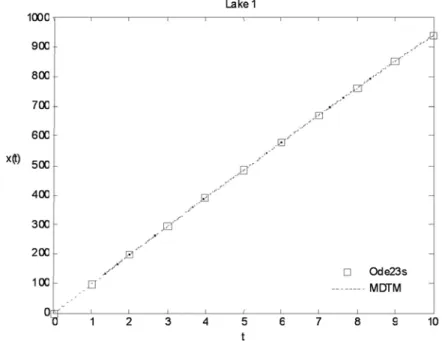
Figure 2. The comparison of the results of () via the two methods for a system of lakes (1)
Figure 2 indicates that the differences among the ode23s with MDTM and the obtained results converge to the ode23s solution and the errors are reduced
Figure 3. The comparison of the results of () via the two methods for a system of lakes (1)
Figure 3 indicates that the differences among the ode23s with MDTM. Ode23s solution is obtained from the solution of MDTM is a good convergence and the error close to zero.
Figure 4. The comparison of the results of () via the two methods for a system of lakes (1)
Ode23s solution is obtained from the solution of MDTM is a good convergence and the error close to zero. As the plots state the amount of the pollutant in lake 1, lake 2 and lake 3 increase.
5. Conclusions
In this paper, the modified difeerential transformation method was used for finding the solutions of nonlinear ordinary differential equation systems such as modelling the pollution of a system of lakes. The obtained solutions are shown graphically. we have presented an after treatment technique for the differen-tial transformation method. Because the Pade´ approximant usually improves greatly the Maclaurin series in the convergence region and the convergence rate, the at leads to a better analytic approximate solution from variational iteration method truncated series We demonstrated the accuracy and efficiency of these methods by solving some ordinary differential equation systems. We use Laplace transformation and Padé approximant to obtain an analytic solution and to im-prove the accuracy of differential transformation method. The reliability of the method and reduction in the size of computational domain give this method a wider applicability. It is observed that The results to get the differential trans-formation method (DTM) applied Padé approximants is an effective and reliable tool for the solution of the nonlinear ordinary differential equation systems con-sidered in the present paper. All the examples show that the results of the present method are in excellent consistency with those obtained by MATLAB ode23s and the modified difeerential transformation method.
References
1. J. Biazar L. Farrokhi and M.R Islam, Modeling the pollution of a system of lakes, Appl. Math. and Comput. 178 (2006) 423—430.
2. ˙Internet: J. Hoggard, Lake Pollution Modeling, Virginia Tech. Available from: http://www.math.vt.deu/pepole/hoggard/links/new/main.html (2008)
3. H.H Robertson, The solution of a set of reaction rate equations, in: J. Wals (Ed.),Numerical Analysis”, An Introduction, Academic Press, London, (1966) 4. F.R Giordano, M.D Weir, Differential Equations: A Modern Approach, Addison Wesley Publishing Company, (1991).
5. J.K. Zhou, Differential Transformation and Its Applications for Electrical Circuits (in Chinese), Huazhong University Press, Wuhan, China, 1986.
6. N. Bildik, A. Konuralp, F. Bek, S. Kücükarslan, Solution of different type of the partial differential equation by differential transform method and Adomian decompo-sition method, Appl. Math. Comput 172 (1) (2006) 551—567
7. V.S. Ertürk, S. Momani, Comparing numerical methods for solving fourth-order boundary value problems, Appl. Math. Comput. 188(2) (2007) 1963-1968.
8. C.K. Chen, S.H. Ho, Solving partial differential equations by two-dimensional differential transform method, Appl. Math. Comput 106 (1999) 171—179
9. I.H.A.H. Hassan, Differential transformation technique for solving higher-order initial value problems, Appl. Math. Comput 154 (2) (2004) 299—311
10. M.J Jang, C.L. Chen, Y.C. Liu, On solving the initial-value problems using the differential transformation method, Appl. Math. Comput. 115 (200) 145—160 11. M.J Jang, C.L. Chen, Y.C. Liu, Two-dimensional differential transform for partial differential equations, Appl. Math. Comput 121 (2001) 261—270
12. M.M.,Al-Sawalha , M.S.M. Noorani, Application of the differential transformation method for the solution of the hyperchaotic Rössler system, Int. Com. in Nonlinear S. and Numeric. Sim. 14 (2009) 1509—1514
13. V.S. Ertürk, differential transformation method for solving differential equations of lane-emden type, Math. Comput.Appl. 12 (3) (2007) 135-139
14. S.J Liao, The proposed homotopy analysis technique for the solution of nonlinear Problems, Ph.D. Thesis, Shanghai Jiao Tong University, (1992).
15. G. Adomian, G., Solving Frontier Problems of Physics: The Decomposition Method, Kluwer Academic, Boston, (1994).
16. A.M Wazwaz, Partial Differential Equations: Methods and Applications, Balkema, Rottesdam, (2002).
17. M. Dehghan , M. Tatari. The use of Adomian decomposition method for solving problems in calculus of variations, Math Prob in Eng. 12 (2006) 653-679
18. D.D. Ganji, A. Rajabi, Assessment of homotopy-perturbation and perturbation methods in heat radiation equations, Internat Commun. Heat Mass Transfer. 33 (2006) 391—400
19. O. Abdulaziz I. Hashim E.S. Ismail, Approximate analytical solution to fractional modified KdV equations, Math. Comput. Model. 49 (2009) 136-145.
20. O. Abdulaziz, I. Hashim, S. Momani, Application of homotopy—perturbation method to fractional IVPs. J. Comput. Appl. Math. 216 (2008) 574-584.
21. MSH Chowdhury, I. Hashim, Solutions of a class of singular second-order IVPs by homotopy—perturbationmethod. Phy. Lett. A 365 (2007) 439—447.
22. MSH Chowdhury, I. Hashim, Solutions of time-dependent Emden—Fowler type equations by homotopy—perturbationmethod. Phy. Lett. A 368 (2007) 305—313. 23. MSH Chowdhury, I. Hashim, O. Abdulaziz, Application of homotopy—perturbation method to nonlinear populationdynamics models. Phy. Lett. A 368 (2007) 251—258. 24. Q.K. Ghori, M. Ahmed A.M. Siddiqui, Application of homotopy perturbation method to squeezing flow of a Newtonian fluid, Int Com. in Nonlinear S. and Numeric. Sim. 8(2) (2007) 179—184.
25. M.A. Rana A.M. Siddiqui Q.K. Ghori, Application of He’s homotopy perturbation method to Sumudu transform. Int Com. in Nonlinear S. and Numeric. Sim. 8(2) (2007) 185—190.
26. A.M. Siddiqui R. Mahmood Q.K. Ghori, Thin film flow of a third grade fluid on a moving belt by He’s homotopy perturbation method Int Com. in Nonlinear S. and Numeric. Sim. 7(1) (2007) 7—14.
27. A.M. Siddiqui M. Ahmed Q.K. Ghori, Couette and Poiseuille flows for non-Newtonian fluids. Int Com. in Nonlinear S. and Numeric. Sim 7(1) (2007) 15—26. 28. J.H. He, “Homotopy perturbation technique”, Comput. Methods Appl. Mech. Eng., 178 (1999) 257—262.
29. J.H. He, A coupling method of a homotopy technique and a perturbation technique for non-linear problems, Internat J. Nonlinear Mech. 35 (2000) 37—43
30. J.H. He, Application of homotopy perturbation method to nonlinear wave equa-tions, Chaos, Solitons Fractals., 26 (2005) 695—700
31. J.H. He, Homotopy perturbation method for bifurcation of nonlinear problems, Internat J. Nonlinear Sci. Numer. Simul., 6 (2005) 207—208
32. M. Dehghan F. Shakeri, Solution of a partial differential equation subject to temperature overspecification byHe’s homotopy perturbation method. Physica Scripta 75 (2007) 778—787.
33. M. Dehghan F. Shakeri, Solution of an integro-differential equation arising in oscillating magnetic fields using He’s homotopy perturbation method. Prog. Electrom. Research. 78 (2008) 361—376.
34. F. Shakeri M. Dehghan, Inverse problem of diffusion equation by He’s homotopy perturbation method. Phy. Letters A. 7 (2007) 551—556.
35. MSH Chowdhury, I. Hashim S. Momani, The multistage homotopy—perturbation method: a powerful scheme for handling the Lorenz system. Chaos, Solit. Fract. 40 (2009) 1929-1937
36. MSH Chowdhury, I. Hashim, Application of multistage homotopy—perturbation method for the solutions of the Chen system. Nonl Analy.: R. W. Appl. 10 (2009) 381-391.
37. L.N. Zhang, J.H He Homotopy perturbation method for the solution of the elec-trostatic potential differential equation. Math. Probl. Engin. 6 (2006) 838-878. 38. ZM. Odibat A new modification of the homotopy perturbation method for linear and nonlinear operators. Appl. Math. Comput. 189 (2007) 746—753.
39. J.H He. Non-perturbative methods for strongly nonlinear problems. Dissertation, de-Verlag im Internet GmbH,Berlin, 2006.
40. J.H He Some asymptotic methods for strongly nonlinear equations. Int. J. M. Phy B. 20(10) (2006) 1141—1199.
41. J.H He New interpretation of homotopy perturbation method. Int. J. M. Phy B.. 20(18) (2006) 2561—256
42. J.H. He, Variational iteration method: a kind of nonlinear analytical technique: some examples, Int. J. Nonl. Mech. 34 (4) (1999) 699—708.
43. J.H He Variational iteration method for autonomous ordinary differential systems, Appl. Math. Comput114 (2000). 115—123
44. J.H He Variational principle for some nonlinear partial differential equations with variable coefficients, Chaos, Solit. Fract. 19 (2004) 847—851
45. Y.C Jiao, Y. Yamamoto, C. Dang, Y. Hao, An aftertreatment technique for improving the accuracy of Adomian’s decomposition method, Comput. Math. Appl,. 43 (2002) 783—798
46. S. Momani, Analytical approximate solutions of non-linear oscillators by the mod-ified decomposition method, Int. J. Modern Phys C. 15 (2004). 967—979
47. E.S. Moustafa, Application of differential transform method to non-linear oscilla-tory systems, Comm. Nonlinear Sci. Numer. Simul. 13 (2008) 1714-1720
48. S. Momani, V.S. Ertürk, Solutions of non-linear oscillators by the modified differ-ential transform method, Comput. Math. Appl. 55 (2008) 833-842.
49. A. Baker, Essentials of Padé Approximants”, Academic Press, London, (1975). 50. A. Baker,. and Graves-Morris,P.,”Pade’ approdmants, Cambridge”, Cambridge University Press,(1996).
51. M. Merdan, Variational iteration method for solving modelling the pollution of a system of lakes, J. Sci. Dumlupınar Univ. 18 (2009) 61-73.
52. M. Merdan, Homotopy perturbation method for solving modelling the pollution of a system of lakes, SDU J. Sci. 4(1) (2009) 99-111.
53. E. Çelik, M. Bayram, Arbitrary order numerical method for solving differential-algebraic equation by Padé series, Appl. Math. Comput. 137 (2003) 57-65.
54. E. Çelik, E. Karaduman, M. Bayram, Numerical solutions of chemical differential-algebraic equations, Appl. Math. Comput. 139 (2003) 259-264.
![Figure 1. System of three lakes with interconnecting channels. A pollutant enters the first lake at the indicated source [4]](https://thumb-eu.123doks.com/thumbv2/9libnet/4731578.89746/2.892.205.671.250.754/figure-lakes-interconnecting-channels-pollutant-enters-indicated-source.webp)