An Analysis of Public Expenditures Using the Median Voter Theorem for Turkey

AN ANALYSIS OF PUBLIC EXPENDITURES USING THE MEDIAN VOTER THEOREM FOR TURKEY

Emin KÖKSAL* ABSTRACT

In this paper, throughout a standard Public Choice model for the demand of public goods, we intend to analyze the public expenditures in Turkey. In doing so, we employ a panel approach to test the median voter theorem at provincial level, over the period 1995-2001. To estimate the parameters in the model with panel data, we use fixed effect estimation specification with least squares method (LS). In addition, to compare the results and justify the reliability of our estimates, we also employ the generalization method of moments (GMM). For a further look, we also advance our study at regional level. Our findings strongly support the theoretical model. Furthermore, our investigation at the regional level suggests sharp differences across the regions.

Keywords: Median Voter Theorem, Public Expenditures, Public Choice Model TÜRKİYE’DEKİ KAMU HARCAMALARININ ORTANCA

SEÇMEN TEOREMİ KULLANILARAK ANALİZİ

ÖZET

Bu çalışmada Türkiye’deki kamu harcamaları, kamu malı talebi için kullanılan standart Kamusal Tercihler modeli aracılığıyla ortanca seçmen teoremi kullanılarak il bazında, 1995-2001 yılları için panel veri yaklaşımıyla test edilmiştir. Panel veri yaklaşımı kullanılırken en küçük kareler yöntemi ile sabit etki tahmini yapılmıştır. Ayrıca, sonuçların güvenilirliğinden emin olmak ve karşılaştırmalı bir gerçekleme yapmak amacıyla genelleştirilmiş momentler yöntemi kullanılmıştır. Çalışma bir adım daha ileriye götürülerek, bölgesel seviyede de yenilenmiştir. Bulgular teorik modeli güçlü bir biçimde desteklemektedir. Ayrıca, bölgesel düzeydeki analizler, bölgeler arasındaki çarpıcı farkı da ortaya koymaktadır.

Anahtar Sözcükler: Ortanca Seçmen Teoremi, Kamu Harcamaları, Kamusal Tercihler Modeli

*

Bahçeşehir Üniversitesi, İktisadi ve İdari Bilimler Fakültesi, Beşiktaş, İstanbul, E-mail: ekoksal@bahcesehir.edu.tr

INTRODUCTION

Analysis of public expenditures constitutes a central issue in the public economics and public finance literature. Considering the public expenditures in the form of publicly supplied goods and services, a series of issues has been addressed. Basically, the cost of those goods and services is provided by the community, and the demand of those goods and services decided collectively (Bergstrom and Goodman, 1973). Although those issues refer to problematical matters, having information about the public good demand of the individuals, hence the community’s, may be useful in many context. For instance, it may be convenient to estimate the possible effects of demographic and economic changes on the public goods to be provided. Or it may be useful to get information about the degree of publicness of the provided goods, in order to ensure efficiency.

In this paper, throughout a standard Public Choice model for the demand of public goods based on median voter theorem, we intend to analyze the public expenditures in Turkey. In doing so, we employ a panel approach to test the median voter theorem at provincial level over the period 1995-2001. Although such a study at cross-sectional level was conducted by Pınar (2001), the writer investigates local government (municipalities) expenditures. However, considering the dominance of central government rather than local governments in Turkey, we employ the expenditures executed through consolidated budget.

To estimate the parameters in the model through panel data, we use fixed effect estimation specification with least squares method (LS). In addition to compare the results and justify the reliability of our estimates, we also employ generalization method of moments (GMM). For a further look, we also advance our study at regional level. Our findings strongly support the theoretical model. Furthermore, our investigation at the regional level suggests sharp differences across regions.

The rest of the paper is organized as follows: While the first section briefly summarizes the theoretical background, the second section exhibits the model. In the third section we introduce the data and in the fourth, we deal with the estimations and their results. Finally, the fifth section consists of concluding remarks.

THE SIGNIFICANCE AND THE EMPIRICS OF THE MEDIAN VOTER THEOREM

The expenditures of private goods are determined in markets through price mechanisms. However, expenditures on public goods are non-market issues and determined through a political process. One of the disciplines exclusively dealing with this issue is the Public Choice Theory, which can be defined as “the economic study of non-market decision-making or, simply the application of economics to political science” (Mueller, 1976: 395).

In public choice theory, it is assumed that decision-making in a political process is executed through a political-exchange, called catallaxy, within the parties of this process. As in exchange in the market between sellers and buyers for private goods, for public goods there exists also a political exchange for the provision. According to Buchanan (1985), politics can be considered as an institution for exchange, like markets. Throughout political exchange individuals of a community try to execute their objectives which they cannot execute efficiently without any collective action. As he mentioned clearly, through political exchange, individuals decide their demand for their collective needs, such as justice, security, education, etc., and their contribution for the provision of these publicly provided goods.

In this context, the median voter model appears as a useful tool for the Public Choice Theory. It is useful to provide a formal explanation for the expenditure level on public goods. Based on the model, median voter theorem suggests that, if the individuals in a community are ranked according to their most preferred levels of public good expenditure, the most preferred level of the individual at the median will emerge as the determinant, in case of a referendum based on majority voting (Rosen, 1999). In other words, outcome of a majority voting procedure in a community will reflect the preferences of the median voter.

However, the validity of the median voter theorem requires an assumption of single peaked preferences. As long as the single peakness assumption is violated, result of the majority voting becomes unstable. Certain restrictions may be applied for this problem. For instance, when we restrict choices for a level of single public good the result usually indicate single-peaked preferences (Kramer, 1973). On the other hand, restrictions for one issue at each time may also ensure the single-peaked preferences (Slutsky, 1975). Furthermore, under some assumptions the

theorem has been proofed in multi-dimensional cases (Mueller, 2003: 67-72).

Although median voter model has some imperfections, it provides a useful framework for the empirical studies which aim to investigate the demand of public goods. In most of these empirical studies, the demand of public goods can be computed by examining how the quantity of public goods depends on the relative price per unit of public good, and the median voter’s income.

Earlier studies by Borcherding and Deacon (1972) and Bergstrom and Goodman (1973) represent a very useful framework for both theoretical and empirical examination of local public spending. Both studies are based on demand analysis of local public goods throughout estimating the median voter’s (identified by median income) demand for the public good. In both studies, the median voter assumed to maximize their utility by consuming private and public goods under the constraint of their budget. In both studies the empirical results suggest significant and expected empirical evidences.1

Some of the studies focus on the relevance of the median voter model. One of those refined studies belongs to Holcombe (1989). Holcombe’s thesis is that, the median voter model can be used as a foundation to understand the public sector demand, like the pure competition in private sector. And, according to the writer, the fundamental model can be extended through various complications, such as multi-peaked preferences. After reviewing strong arguments both empirically and theoretically, Holcombe suggests that median voter theorem is a good approximation of demand aggregation in the public sector for various issues.

On the other hand, Mueller (2003) emphasizes on comparative empirical tests for the median voter model. The writer argues that empirical tests should be based on some comparison of performance of spending models with mean and median variables, such as income and tax share. Pommerehne and Frey (1976) and Pommerehne (1978) can be cited as the major empirical works to compare the performances of the models with mean and median variables. While the study by Pommerehne and Frey (1976) provides empirical evidences on behalf of the spending models with median variables, Pommerehne (1978) gives further information that suggests median income performs well in direct

1 _{In both empirical studies (Borcherding and Deacon, 1972; Bergstrom and Goodman,} 1973) income elasticity is positive and significant; price elasticity is negative and significant, which respect to the median voter theorem.

democracy governments, but in a representative government it does not sustain a distinguished performance against the models with mean income variables.

THE MODEL

For a pure public good, the median voter’s problem can be written as; ) Q , y ( U

U

max

Q , y = (1) subject to

Q

p

y

p

I

_m

=

_y

+

τ

_Q

where

y

,

q

,

p

_yand

p

_Qare defined as quantity of private good, quantity of public good and their prices, respectively.

τ

and

I

_m

represent tax share and income of median voter, respectively. Also,

Q

implies the total provision of public good.

The first order conditions associated with the above maximization problem suggest the following demand function for the public good

) I , p , p ( Q Q= _y

τ

_{Q m} (2)

The demand function in equation (2) refers to the demand of a pure public good.2 However, certain public goods may be partially rival; for this intermediate case we barrow a device from Borcherding and Deacon (1972: 893) which implies to the level of public good available for consumption, α N / Q * Q = (3)

where

0

≤

α

≤

1

, and

N

represents population. Note that in extreme cases, when

α

=

0

and

α

=

1

_{the good is purely public and}

private, respectively. In intermediate cases, the good exhibits impure characteristic, in terms of its rivalness in consumption.

Equation (3) allows us to find a price for an ordinary demand function for

Q

*

as

τ

p

_Q

N

α, which indicates price of public goods

2 _{Pure public goods are the goods neither rival nor excludable in consumption. Non-rivalry} in consumption refers to cases for which one person’s consumption does not reduce or prevent another person’s consumption. Non-excludability, implies that it is either or prohibitively costly to exclude any individual from the benefits of the public good.

available for consumption. Then, the demand function for

Q

*

can be written as

)

,

,

(

*

*

Q

p

_y

p

_Q

N

I

_m

Q

=

τ

α (4)

By assuming a constant elasticity demand function, borrowing from Bergstrom and Goodman (1973), one can derive the demand function for

*

Q

as; φ η δ α

τ

p

Q

N

I

m

p

y

c

Q

*

=

(

)

(5)

And, substituting equation (5) in equation (3) gives us the total level of purchased

Q

as λ φ η δ

τ

p

I

p

N

c

Q

=

(

Q

)

m y (6) where λ=α(1+δ ).

In logarithmic form equation (6) becomes

N

p

I

p

c

Q

ln(

_Q

)

ln

_m

ln

_y

ln

ln

=

+

δ

τ

+

η

+

φ

+

λ

(7) The above equation is very helpful in our context in many ways. First of all, the estimation of the coefficients (with the addition of an error term) gives us the elasticity measures of each variable. The price elasticity of demand (

δ

), income elasticity of demand (

η

), and elasticity of private good prices (

φ

) can be identified. Moreover, it has to be emphasized that increase in population will influence the public expenditure through tax share and degree of publicness. More clearly, recalling λ=α(1+δ ) where

α

is the rivalry parameter, as the population increases tax share will decrease at a magnitude depending on the rivalry of the public expenditures.

Although equation (7) exhibits a useful characteristic for an empirical estimation, the price elasticity has been masked by the effects of tax share (

τ

). Since

τ

represents the median voter’s share of the cost of one unit of public good, empirically measuring

τ

refers to a problematic issue. Thus, we follow Dudley and Montarquette (1981) and assume an equal cost sharing among the population, which implies

N

/

1

=

τ

₍₈₎

Then, substituting equation (8) in equation (7), transforms the equation into form as;

N ln p ln I ln p ln c Q ln = +

δ

_Q +

η

_m+

φ

_y +

θ

(9) where

δ

δ

α

θ

=

(

1

+

)

−

_.

Thus, equation (9) becomes practical to serve us as a model to estimate, with the addition of an error term. This econometric specification will serve us as the first model to estimate the important determinants of public expenditure.

DATA

In most of the seminal papers (Bergstrom and Goodman, 1973; Borcherding and Deacon, 1972; Dudley and Montarquette, 1981) and in the Turkey-specific study (Pınar, 2001), the median voter demand functions were estimated through cross-sectional data. Conversely, we used panel data with 79 provinces3 _{over the seven year period of} 1995-2001. The most obvious conveniences of this approach, which distinguish it from the cross-sectionals, may be interpreted in two ways. First, it provides a larger number of observations through adding the time dimension. Second, we obtain both inter-province and intra-province variations for all variables.

The data used in this paper has been collected from three official resources: Turkish Statistical Institute (TURKSTAT), Central Bank of Republic of Turkey (CBRT) and General Directorate of Public Accounts (GDPA). From those data sources, we sought the required data with an annual period for each 79 provinces in Turkey, to create a balanced panel data set. Although we would have liked to estimate with a larger number of observations, we have been restricted by the lack of time-series regional statistics in many variables. Thus, we had to restrict our study with a period of seven years, 1995-2001. In other words, our number of observation has restricted us with 553 observations. In many contexts, this observation number may be acceptable.

To empirically measure the dependent variable, quantity of public good (

Q

), we use consolidated budget expenditures for each province deflated by public sector price deflator (1994=100). The consolidated budget consists of both general and annexed budgets. By definition, while an institution which is financed by general budget provides pure public goods, and institutions with annexed budgets provide semi or impure public goods, such as education. Although the consolidated budget has ignored the special budgets for local authorities, such as municipalities, as Pınar (2001) suggested, local authorities prefer relying

3 _{We exclude the provinces, Duzce and Osmaniye, because of missing data for earlier years} of the period.

on central government rather than local revenue sources as a way of tax related political risks. Facing with this Turkey-specific reality, we argued that expenditures financed by consolidated budget may be a better measure for the quantity of public good.

On the other hand, none of the data sources provide the identity of the voter with median preferences for the public good; hence, their income (

I

_m) is not known. In earlier studies, e.g. Bergstrom and Goodman (1973), have argued that there would be some possible systematic errors for particular choices of proxies for the median voter’s income. However, following Murdoch, Sandler and Hansen (1991: 627), we argue that for each province we can place a proxy variable that is highly correlated with the income of the median voter, in a panel data which consists partially by time series data. The most conventional one may be the mean income, based on the results suggested by Pommerehne (1978)4. Hence, we use GDP per person. We prefer GDP per person in current prices for each province, in order to capture more the price related issues.5

For the unit prices of public (

p

_Q) and composite private goods (

y

p

), we use public sector price index (1994=100) and consumer price index (1994=100), respectively. While the former is unique for each year for all provinces, the latter variable is available for some provinces and for all geographical regions. For public goods, it can be reasonable to assume that most of the supplies purchased by provinces are subject to the national market. There is no objection to use a unique indicator for each region. For instance, considering the salaries for officials, they are all the same across countries, excluding some side payments. However, we cannot argue the same thing for private goods, since local factor prices are more influential on private goods.

The data for the population consists of mid-year population estimations, which are calculated based on two consecutive census’ definite results for each province. The complete list of variables is displayed in Appendix 1.

4 _{As mentioned above, Pommerehne (1978) suggested that median income performs well in} direct democracy governments, but in a representative government it does not sustain a distinguished performance against the models with mean income variables.

5 _{Current GDP is preferred because prices in equation (9) later will be represented by price} indexes (public sector and consumer price indexes) which are closely related with the deflator used for real GDP.

ESTIMATION AND EMPIRICAL RESULTS

In this section, the model outlined in section 3 will be estimated with two alternative methods, least squares (LS) and generalized method of moments (GMM), throughout our panel data. Existence of alternative estimation method aims to compare and justify the reliability of our estimation.

However, before starting the estimations, checking for the muticollinearity problem gives us high pair-wise correlations among some regressors. The indexes chosen for the unit price of composite private good and public good suggest high correlations with each other and with GDP per person, which refers to a proxy of median voter’s income.6

In order to construct a reliable econometric specification, this problem forces us to drop at least one of the price index variables from the model. Considering the price of public good as an essential element of the model, we drop the index used for price of private goods. At first sight, this action can be seen as a specification bias which implies incorrect specification of the theoretical model. However, as soon as we assume that public goods are not substitutable with private goods, we can manage the problem. In fact, most of the goods and services, which are provided publicly, have not any private alternative. Then our econometric specification will not refer to any specification bias against the theoretical model.

Another important issue, which will shape our specification, comes from the AR process. Both our doubt and test showed that the dependent variable has an AR(1) process. Considering the budget principal, which implies appropriation of annual allowances and cancellation of unexpended appropriations, AR(1) process may be legitimated in reality.

Thus the main econometric specification to estimate appears as;

t i 1 t i t i t i m t i Q t i

c

ln

p

ln

I

ln

N

ln

Q

u

Q

ln

=

+

δ

+

η

+

θ

+

−

+

, (10) where subscripts show the cross-sections and superscripts imply time series.

Our main intention is to discover that our estimates of income elasticity are significant and positive, and the estimates of price elasticity are significant and negative. Although the estimates of population elasticity are related with price elasticity parameter and the crowding

6 _{See Appendix 2.}

parameter,7 _{its expected sign must be positive. Considering the earlier} studies and assuming that all public goods are not pure then, this expectation can be legitimized.

In estimation with LS method, we use fixed effects specification to exploit the richness of the data. Through using fixed effect specification, each cross-sectional unit, here each province has its own intercept value. Thus, by controlling effectively the cross-section effects, we can deal more with the variable of interests. The results are presented in Table 1. Table 1: Fixed Effect Estimation with LS

Estimated parameter Coefficient Std. Error t-Statistic Price elasticity -0.52*** 0.04 -12.42 Population elasticity 0.55*** 0.06 9.75 Income elasticity 0.51*** 0.05 10.67 Elas. of preceding level 0.54*** 0.06 9.40

R-squared: 0.99 Durbin-Watson stat: 2.11 Number of obs: 474

Before interpreting the results some econometric issues must be mentioned about the estimation. First, the results are cross-sectional weighted GLS estimates, to allow heteroscedasticity in a relevant dimension. Second, to attain robust standard errors we employ White’s heteroscedasticity–correction.

The results are completely consistent with the theoretical model, in terms of their significances and their signs. In earlier studies, i.e., Bergstrom and Goodman (1973) and Borcherding and Deacon (1972), it is reported that income elasticities are less than one and price elasticities in the range of -0.2 to -0.6. Our results are robust and remain in the mentioned intervals.

However, as mentioned earlier, population elasticity consists of price elasticity parameter and the crowding parameter. Considering the estimated measures in Table 1, one can calculate the crowding parameter as 0.07, approximately. This refers to the characteristic of the public goods with a high degree of publicness. In other words, the provided goods are almost non-rival, or pure.

The confirmation of theory across the country motivates us to make some additional tests at regional level. In fact, we were curious

7 _{Recall that}

θ

=

α

₍

₁

+

δ

₎

−

δ

about the behavior of the model with different subgroups. Accordingly, we divide the country into three zones, taking into account the level of GDP per person. Accordingly, the first zone consists of the regions Marmara and Aegean (MAR-AEG). The second zone consists of Central Anatolia, Black Sea and Mediterranean (CEN-BLS-MED). And the third zone consists of East and South East Anatolia (EAS-SEA).

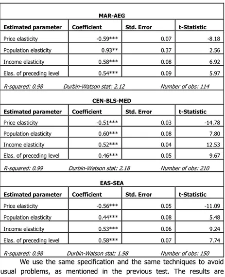
Table 2: Fixed Effects Estimation with LS for zones

MAR-AEG

Estimated parameter Coefficient Std. Error t-Statistic Price elasticity -0.59*** 0.07 -8.18 Population elasticity 0.93** 0.37 2.56 Income elasticity 0.58*** 0.08 6.92 Elas. of preceding level 0.54*** 0.09 5.97 R-squared: 0.98 Durbin-Watson stat: 2.12 Number of obs: 114

CEN-BLS-MED

Estimated parameter Coefficient Std. Error t-Statistic Price elasticity -0.51*** 0.03 -14.78 Population elasticity 0.60*** 0.08 7.80 Income elasticity 0.52*** 0.04 12.53 Elas. of preceding level 0.46*** 0.05 9.67 R-squared: 0.99 Durbin-Watson stat: 2.18 Number of obs: 210

EAS-SEA

Estimated parameter Coefficient Std. Error t-Statistic Price elasticity -0.56*** 0.05 -11.09 Population elasticity 0.44*** 0.08 5.48 Income elasticity 0.53*** 0.06 9.24 Elas. of preceding level 0.58*** 0.07 7.74 R-squared: 0.98 Durbin-Watson stat: 1.98 Number of obs: 150

We use the same specification and the same techniques to avoid usual problems, as mentioned in the previous test. The results are exhibited in Table 2, for each zone.

At first sight, the elasticity measures do not exhibit a derogative view, in terms of their signs and significances. However, a further

investigation helps us to state the differences. First, while the income elasticity for EAS-SEA and CEN-BLS-MED follow the same pattern for the general test across the country, the income elasticity for MAR-AEG is significantly greater than the other estimates. Second, the same pattern can be observed for the price elasticities; again the elasticity for MAR-AEG is greater than the other estimates.

More interestingly, the elasticity of population is the most variant in both estimations. Particularly, extreme values are obtained for MAR-AEG and EAS-SEA districts, 0.93 and 0.43, respectively. Those extreme values also suggest other extreme values for the crowding parameter. The calculations give us the crowding parameters as 0.84 for MAR-AEG and -0.28 for EAS-SEA.8

The parameter for MAR-AEG can be interpreted through considering the demographic situation in the zone. Since the population concentration is relatively high in the district, it may be argued that as the population increases the rivalness degree of the provided good increases. Alternatively, as Bergstrom and Goodman (1973) argued, there appear to be no economies of scale to larger provinces in the provision of the public good.

However, the estimated parameter for EAS-SEA, is quite interesting and perhaps, it has to be evaluated as economically nonsense. An alternative interpretation can concern the externalities issue, because of non-rival and non excludable characteristic of public goods. But details of this interpretation may go beyond the frontiers of this paper. However, it must be noted that the crowding parameter increases as the city sizes increase; at least in the sample for this study.

Finally, in order to show the robustness and consistency of the estimated coefficient by LS method, we employ the GMM method. In fact, GMM for a panel data may be a useful tool for our data, with large number of cross-sections and short time series.

For the GMM estimation we use the same econometric specification defined in equation (10). As in the estimation with LS method, we use fixed effects specification. Also, for the heteroscedasticity case, cross-sectional weighted GLS and White’s heteroscedasticity–correction are employed. In addition, instruments list for the GMM estimation, which consists of lag values of regressors, is arranged. The results are shown in Table 3.

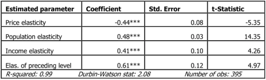
Table 3: Fixed Effects Estimation with GMM

Estimated parameter Coefficient Std. Error t-Statistic Price elasticity -0.44*** 0.08 -5.35 Population elasticity 0.48*** 0.03 14.35 Income elasticity 0.41*** 0.10 4.26 Elas. of preceding level 0.61*** 0.12 4.97 R-squared: 0.99 Durbin-Watson stat: 2.08 Number of obs: 395

At first sight, the significance and the signs of the coefficients completely confirm the results that we obtained through LS. However, the value of the coefficients has decreased almost 20 percent, except the coefficient of the lagged dependent variable. Calculations of the estimated crowding parameter also give similar value as the LS, 0.77.

Although GMM provides a useful framework for the comparison of the common estimators, it is a large sample estimator. As we are aware of this phenomenon, we do not try to compare the estimated values of the coefficients from the test on zones. In panel data, as the number of cross-sections, hence the number of observations decreases, the efficiency of the GMM estimators also decreases.

CONCLUDING REMARKS

In this paper we have employed the median voter model of Public Choice Theory as a tool to analyze the government expenditures in Turkey across the provinces. We have tested the model using fixed effect estimation both at country and region level through LS method. Also a comparison for the validity of the estimated parameters has been checked with an alternative estimation method, GMM. Both estimation results suggest strong evidences for the confirmation of the theoretical model across the country within the mentioned period.

Income elasticity is positive and significant as expected, in all estimations. The estimates remain the values that are reported in other empirical studies. However, the estimation at the regional level gives us some clues, which suggest that income elasticity is decreasing gradually throughout west to east. This evidence may be interpreted in many ways. For instance, one may argue that urbanization plays a major role for the income elasticity. Thus, it would be interesting to measure the effect of urbanization. But, we have not encountered a suitable standard source of data to test this phenomenon for our sample. Another

argument may be on the grounds of politics, but we would not like to make speculations in the limited scope of this paper.

Population elasticity and price elasticity may be elaborated commonly, since their estimated values define the crowding parameter. As expected, the price elasticity is negative. That means public good is a normal good. The population elasticity is positive, which is consistent with the theory. However, while the price elasticity has not varied across regions, the population elasticity, hence the crowding parameter, are terribly different. This dispersion should be interpreted carefully, since we have a strong assumption which implies equal tax share among the population (

τ

=

1

/

N

). However, one can argue that in eastern regions, by interpreting the negative value of crowding parameters as close to zero, there should be large economies of scale in terms of benefits of publicly provided goods.

Finally, there are some comments about this work that we wish to address here. First of all, it may be argued that time series that we have used might not be long enough to analyze the dynamic effects for the elasticities. Although our balanced panel fit the model better than the cross-sectional one, more time series may increase the reliability of the model. Secondly, throughout the study, our analysis ignores the political considerations about the public expenditures; but as mentioned earlier, this sort of discussion is further than the scope of this paper.

REFERENCES

Bergstrom, T. & Goodman, R.P. (1973). Private Demands for Public Goods. American Economic Review, 63(3), 280-296.

Borcherding, T.E. & Deacon, R.T. (1972). The Demand for Services of Non-Federal Governments. American Economic Review, 62(5), 891-901.

Buchanan, J.M. (1985). Liberty, Market and State: Political Economy in 1980s. New York: New York University Press.

Dudley, L. & Monmarquette, C. (1981). The Demand for Military Expenditures: An International Comparison. Public Choice, 37(1), 5-31.

Holcombe, R.G. (1989). The Median Voter in Public Choice Theory. Public Choice, 61, 115-125.

Kramer, G. (1973). On a Class of Equilibrium Conditions for Majority Rule. Econometrica, 42(2), 285-297.

Mueller, D.C. (1976). Public Choice: A Survey. Journal of Economic Literature, 14(2), 395-433.

Mueller, D.C. (2003). Public Choice III. Cambridge: Cambridge University Press.

Murdoch, J.C., Sandler, T. & Hansen, L. (1991). An Econometric Technique for Comparing Median Voter and Oligarchy Choice Models of Collective Action: The Case of the NATO Alliance. The Review of Economics and Statistics, 73(4), 624-31.

Pınar, A. (2001). A Cross-Section Analysis of Local Public Spending in Turkey. METU Studies in Development, 28, 203-218.

Pommerehne, W.W. (1978). Institutional Approaches of Public Expenditures: Empirical Evidences from Swiss Municipalities. Journal of Public Economics, 9, 163-201.

Pommerehne, W.W. & Frey, B.S. (1976). Two Approaches to Estimating Public Expenditures. Public Finance Quarterly, 4, 163-201.

Rosen, H.S. (1999). Public Finance (5th edition). New York: McGraw Hill. Slutsky, S. (1975). A Voting Model for the Allocations of Public Goods:

Existence of Equilibrium. Journal of Economic Theory, 11(7), 292-304.

APPENDICES

Appendix 1: Variables in the Model

Dependent variable

Qi: Consolidated budget expenditure for the ith _{province, with the prices of 1994} Independent variables

PQi: deflator for public sector (1994=100)

Imi: per capita GDP for the ith _{province, in current prices} Pyi: consumer price index for ith _{province (1994=100)} Ni: population of the ith _provinces

Appendix 2: Correlation Matrix of Regressors

lnQ lnIm lnpy lnpQ lnN lnQ 1.000000 lnIm 0.226009 1.000000 lnpy 0.097289 0.913458 1.000000 lnpQ 0.084887 0.803364 0.997743 1.000000 lnN 0.897784 0.152925 0.030702 0.021788 1.000000